“If tension is about pulling and compression is about pushing, then shear is about sliding.”
— J. E. Gordon, Structures: Or Why Things Don’t Fall Down, 1978
The normal stress of the previous chapter came from cutting a bar perpendicular to the load, so that the internal force pointed straight out of the cut surface. Nothing forces us to cut that way. If we instead cut parallel to the load, the internal force lies in the plane of the cut and tries to slide one face of the cut past the other. The internal force per unit area is then called the shear stress, and it is what fails a bolt, a rivet, a weld or a glued lap joint.
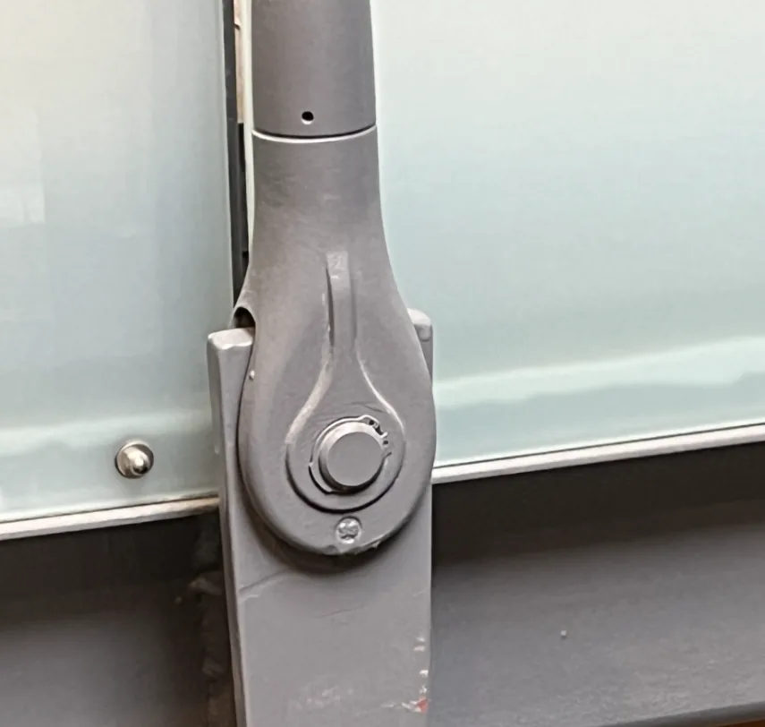
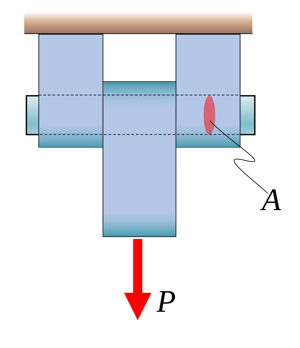
Figure 8.4.1: Rod holding the walkway in the School of Education and Communication. The pin is in double shear.
Denoting the internal force tangential to the cut by \(T\) and the area of the cut by \(A\), the average shear stress is
\[
\boxed{\tau = \frac{T}{A}}
\tag{8.4.1}\]
which has the same form and the same units as 8.3.2. The difference is entirely in the direction: \(\sigma\) acts along the surface normal and \(\tau\) acts in the surface. Since the two are distinguished only by the orientation of the cut, we should already suspect that they are two faces of one object rather than two separate quantities, and Example 2 below makes that suspicion concrete.
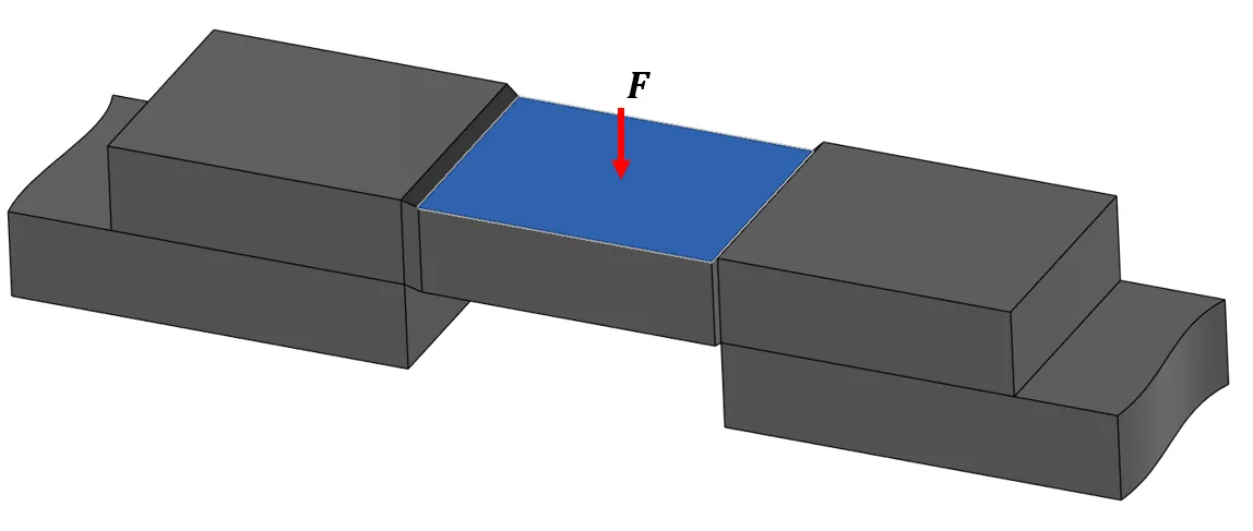
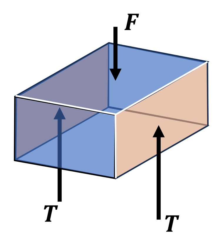
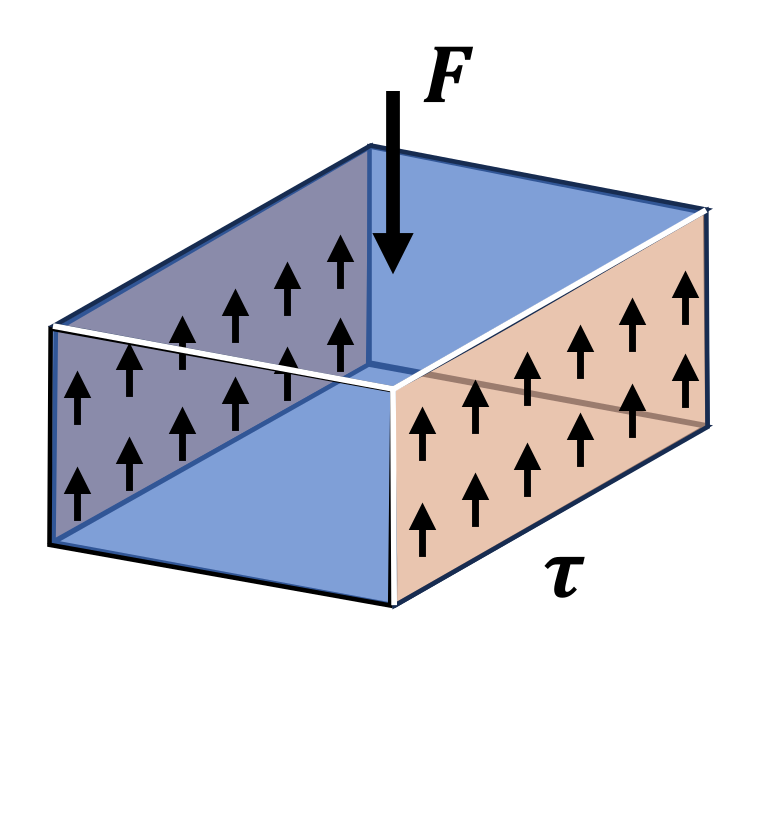
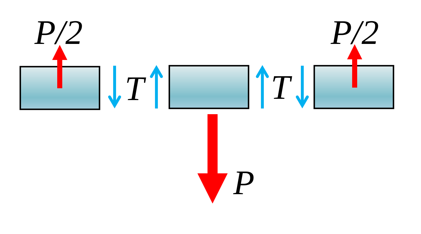
Two arrangements occur so often that they have names. In single shear the joint presents one cut surface, so the pin carries the whole load across a single section. In double shear the joint presents two, and each carries half the load, which halves the stress for the same pin. Figure 8.4.2 shows double shear in its simplest form, a block pushed down between two fixed blocks.
(a) The load case
(b) Free body diagram
(c) Average shear stress
Figure 8.4.2: A block in double shear. The load \(F\) pushes the middle block down between two fixed blocks, and it is cut free along the two faces where it meets them. Each of the two shear planes carries \(T\), so \(T = F/2\), and the average shear stress on each plane is \(\tau = T/A = F/(2A)\).
The free body diagram of the pin shows how many shear planes carry the load.
Example 1: A pin in double shear
A cylindrical pin of cross-sectional area \(A\) joins a clevis to a tongue and carries a force \(P\), as shown in Figure 8.4.3. Determine the shear stress in the pin.
Figure 8.4.3: A pin in a clevis joint.
We isolate the pin. The tongue pushes on it with \(P\) in the middle, and the two arms of the clevis push back with \(T\) each, so equilibrium reads \(P - 2T = 0\).
The two shear planes halve the stress compared to a single-shear joint carrying the same load, which is exactly why clevis joints are preferred wherever the geometry allows them.
Example 2: Stress on an inclined cut
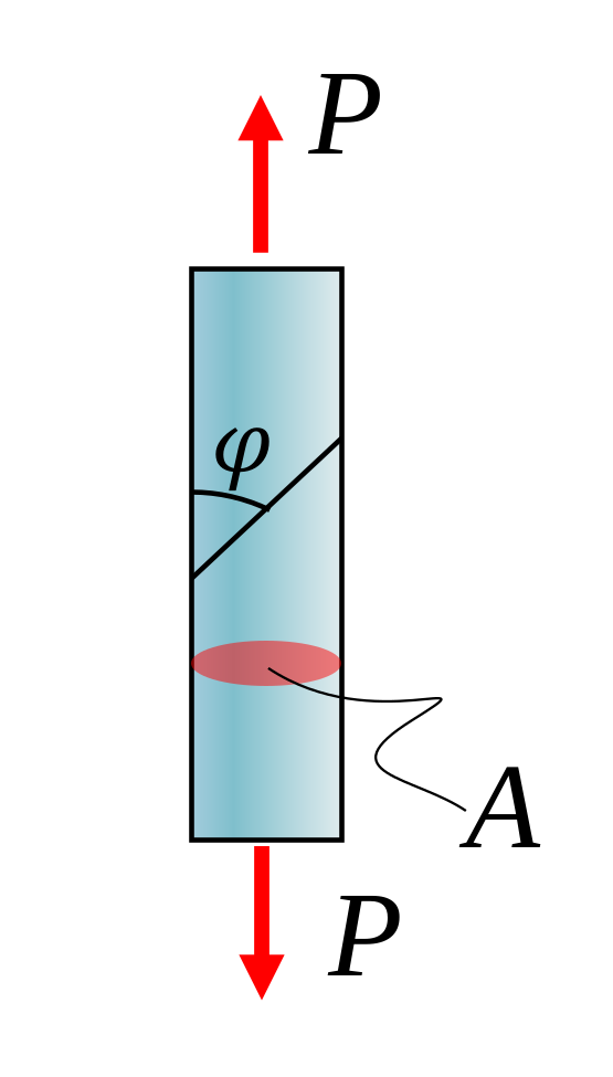
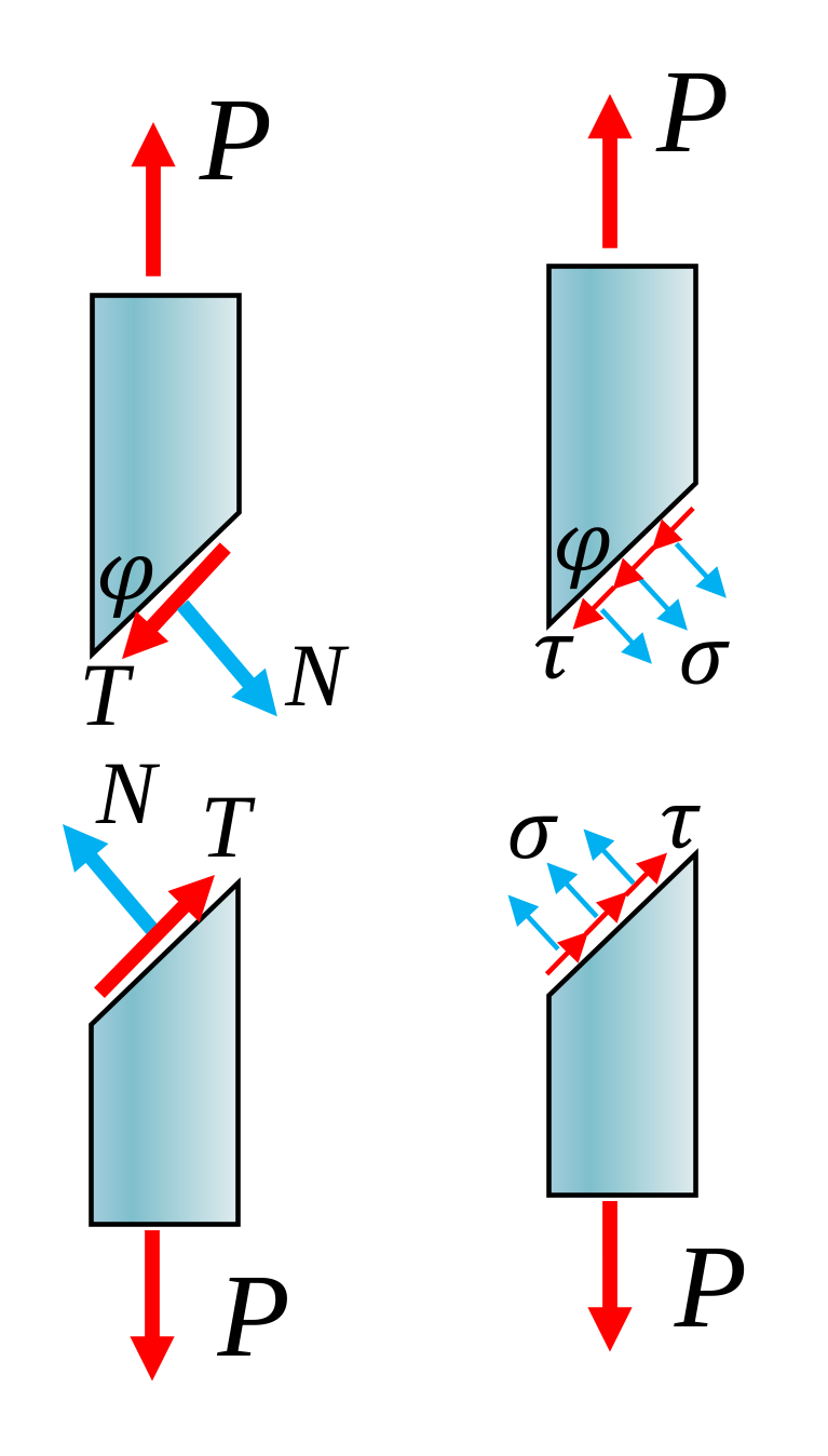
A prismatic bar of cross-sectional area \(A\) is pulled by an axial force \(P\). Cut it at an angle \(\varphi\) to the bar axis, as in Figure 8.4.5 (a), and determine the normal and shear stress on that cut. At which angle is the shear stress largest?
(a) The bar, the cut at the angle \(\varphi\) to its axis and the cross-section \(A\).
(b) The two parts of the bar on either side of the cut, with the internal force as \(N\) and \(T\) (left) and as the stresses \(\sigma\) and \(\tau\) (right).
Figure 8.4.5: A bar in uniaxial tension cut at an angle to its axis.
The inclined cut has area \(A/\sin\varphi\), which grows without bound as the cut approaches the axis. We take the lower part in Figure 8.4.5 (b), with \(x\) across the bar and \(y\) along it, toward the load. The cut makes the angle \(\varphi\) with the axis, so its outward normal and its tangent are
\[
\bm n = [-\cos\varphi, \sin\varphi]^\mathsf{T}, \qquad \bm t = [\sin\varphi, \cos\varphi]^\mathsf{T}
\]
and the internal force on the cut is \(N\bm n + T\bm t\), with \(N\) normal to the cut and \(T\) tangential to it. Equilibrium of the lower part in the two coordinate directions, and the definitions of the two stresses on the cut of area \(A/\sin\varphi\), give four equations for \(N\), \(T\), \(\sigma_\varphi\) and \(\tau_\varphi\),
N, T, varphi, P, A, sigma_varphi, tau_varphi = sp.symbols('N T varphi P A sigma_varphi tau_varphi', real=True)eqs = [sp.Eq(N*sp.sin(varphi) + T*sp.cos(varphi) - P, 0), # equilibrium along the load sp.Eq(-N*sp.cos(varphi) + T*sp.sin(varphi), 0), # equilibrium across the load sp.Eq(sigma_varphi, N/(A/sp.sin(varphi))), sp.Eq(tau_varphi, T/(A/sp.sin(varphi)))]sol = sp.solve(eqs, [N, T, sigma_varphi, tau_varphi], dict=True)[0]sol = {k: sp.simplify(v) for k, v in sol.items()}sol | la
\[ \begin{aligned}
N &= P \sin{\left(\varphi \right)} \\[9.0pt]
T &= P \cos{\left(\varphi \right)} \\[9.0pt]
\sigma_{\varphi} &= \dfrac{P \sin^{2}{\left(\varphi \right)}}{A} \\[9.0pt]
\tau_{\varphi} &= \dfrac{P \sin{\left(2 \varphi \right)}}{2 A}
\end{aligned} \]
The two stresses on the inclined cut are therefore
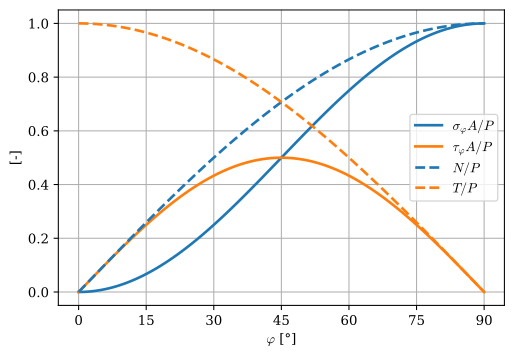
and the double angle in the second expression tells us immediately where the maximum lies. Plotting both over the full range of cut angles makes the behaviour clear.
Code
phi_deg = sp.symbols('phi_deg', real=True)in_degrees = {varphi: sp.pi*phi_deg/180} # plot against the angle in degreesfig, ax = plt.subplots(figsize=(6, 4))# each force in the colour of the stress it gives, stresses solid and forces dashedfor expr, style, col, lbl in ((sol[sigma_varphi]/P*A, '-', 'C0', r"$\sigma_\varphi A / P$"), (sol[tau_varphi]/P*A, '-', 'C1', r"$\tau_\varphi A / P$"), (sol[N]/P, '--', 'C0', r"$N / P$"), (sol[T]/P, '--', 'C1', r"$T / P$")): fplot(sp.simplify(expr).subs(in_degrees), (phi_deg, 0, 90), ax=ax, linewidth=2, linestyle=style, color=col, label=lbl)ax.set_xlabel(r"$\varphi$[°]")ax.set_xticks(range(0, 91, 15))ax.set_ylabel("[-]")ax.grid(True)ax.legend()plt.show()
Figure 8.4.6: The stresses (solid) and the forces (dashed) on a cut inclined at \(\varphi\) to the axis of a bar in uniaxial tension, the stresses in units of \(P/A\) and the forces in units of \(P\).
The shear stress peaks at \(\varphi = \pi/4\), that is at \(45^\circ\), where it reaches \(P/2A\), half the maximum normal stress. The normal stress meanwhile grows monotonically and reaches its own maximum \(P/A\) on the perpendicular cut at \(\varphi = \pi/2\), where the shear stress has fallen to zero.
We applied a single axial load and made no change whatsoever to the bar or to the loading, yet by choosing a different cut we obtained a different pair of stresses. A cut at \(90^\circ\) sees pure tension, a cut at \(45^\circ\) sees the largest shear the bar will ever experience, and every angle in between sees a mixture. The stress at a point is therefore not one number but a rule that assigns a traction to every possible cut direction, and the mathematical object encoding such a rule is a tensor. We construct it in Chapter 8.7, where 8.4.2 reappears as a special case of the transformation of the stress tensor under rotation.
The physical consequence is visible in any tensile test of a ductile metal. The specimen is pulled axially but yields along planes inclined at roughly \(45^\circ\), because plastic slip in metals is driven by shear rather than by tension. A brittle material such as chalk instead fails on the plane of maximum normal stress, straight across.
Example 3: Dimensioning two pins
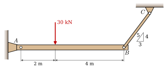
The rigid beam in Figure 8.4.7 is pinned at \(A\) and supported by a link at \(B\) inclined so that its direction has components \((3, 4)/5\). A load of \(30~\text{kN}\) acts \(2~\text{m}\) from \(A\), and the link attaches \(6~\text{m}\) from \(A\). The maximum allowable shear stress in the pins is \(180~\text{MPa}\) and the factor of safety is \(1.5\). The pin at \(A\) is in double shear and the pin at \(B\) is in single shear. Determine the required pin diameters.
Figure 8.4.7: The beam is pinned to the wall at \(A\) and held at \(B\) by the link \(BC\), whose direction has the slope \(4/3\).
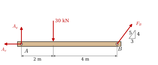
The free body diagram of the beam gives three equilibrium equations for the three unknown reaction components. Taking moments about \(A\) isolates the link force \(F_B\) immediately, after which the two force equations give the components at \(A\).
Figure 8.4.8: Free body diagram of the beam.
With the load \(F_G = 30~\text{kN}\), \(x\) to the right, \(y\) up and counterclockwise moments positive, and with lengths in metres, the free body diagram gives
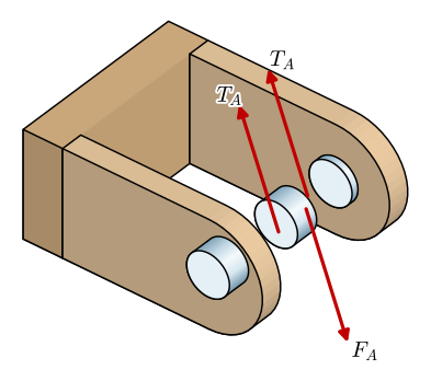
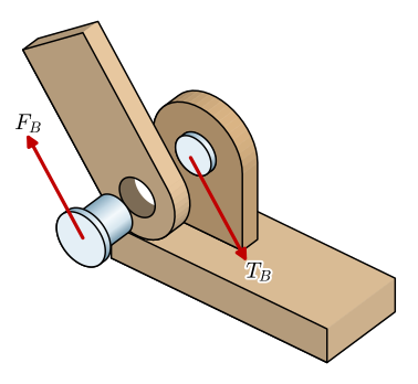
The pin at \(A\) carries \(F_A\), and since it sits in double shear the force splits between two sections, \(T_A = F_A/2\). The pin at \(B\) carries the full link force across a single section, \(T_B = F_B\).
Figure 8.4.9: The pin at \(A\) runs through both arms of the clevis on the wall, with the beam, not drawn, between them. Cut free at the two shear planes, the middle of the pin carries the push \(F_A\) of the beam and \(T_A\) on each cut, so \(T_A = F_A/2\).
Figure 8.4.10: The joint at \(B\) pulled apart along the pin. The eye of the link sits beside the bracket on the beam, so the pin is cut at one plane only, and the piece in the eye carries the link force \(F_B\) and \(T_B = F_B\) on its cut.
With the allowable shear stress \(\tau_{\text{allow}} = 180/1.5 = 120~\text{MPa}\), each diameter follows from setting the actual shear stress on one section equal to the allowable one,
Rounding upward, the pin at \(A\) needs at least \(11~\text{mm}\) and the pin at \(B\) at least \(12~\text{mm}\). In practice we would fit \(12~\text{mm}\) pins in both positions. The slightly heavier pin at \(A\) costs almost nothing, whereas two different pin sizes in one assembly cost a second tool, a second stock item and a chance to assemble the joint wrongly.
Note that the pin at \(B\) ends up larger despite carrying a smaller force, \(12.5~\text{kN}\) against \(21.4~\text{kN}\). The double shear at \(A\) is what makes the difference, and it illustrates that the load path through a joint matters as much as the magnitude of the load itself.
Example 4: A pinned lap joint
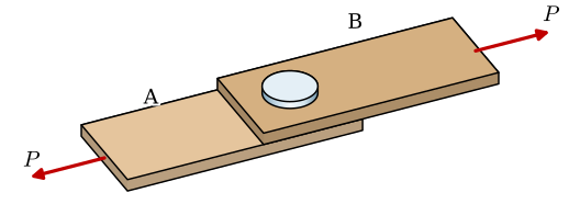
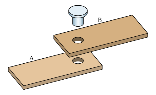
Two steel plates overlap and are joined by a single pin through the middle of the overlap, as in Figure 8.4.11. The plates are \(w = 40~\text{mm}\) wide and \(t = 5~\text{mm}\) thick, the pin has the diameter \(d = 12~\text{mm}\), and the centre of the hole lies \(e = 20~\text{mm}\) from the end of each plate. The joint carries the tensile load \(P = 20~\text{kN}\). The plates are of S355 steel, \(\sigma_y = 355~\text{MPa}\), and the pin of property class 8.8, \(\sigma_y = 640~\text{MPa}\). Determine the factor of safety against each way the joint can fail, and find the one that governs.
(a) The joint in tension.
(b) The joint taken apart along the pin.
Figure 8.4.11: Two plates \(A\) and \(B\) joined by one pin and pulled apart by \(P\).
The load passes from plate \(A\) through the pin into plate \(B\), and every part of that path can fail. Plate \(A\) is pulled to the left by \(P\) at its far end and held by the pin, which pushes on the half of the hole toward the plate end. Figure 8.4.12 shows the four ways the plate can fail, and plate \(B\) is loaded the same way in the opposite direction.
(a) Tension on the net section through the hole.
(b) The stress concentrated at the edge of the hole.
(c) Bearing of the pin on the hole.
(d) Tear-out of the end between two shear planes.
Figure 8.4.12: The four ways plate \(A\) of the lap joint can fail, seen from above.
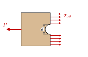
Away from the hole the plate carries \(P\) on its whole cross section \(Wt\), the gross section. At the hole the material is missing, and the same force passes through the two ligaments beside it, the net section\((w - d)t\) of Figure 8.4.12 (a),
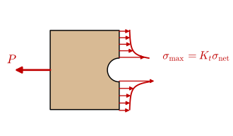
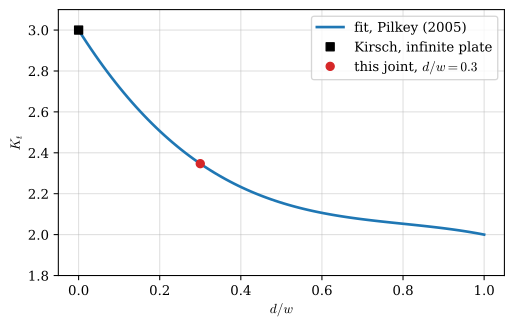
The net section stress is an average. The lines of force bend around the hole and crowd together at its edge, so the stress there is higher than the average, as sketched in Figure 8.4.12 (b). The ratio of the peak to the net section stress is the stress concentration factor\(K_t\), which depends only on the geometry. For a round hole in a plate of finite width, a curve fitted to the tabulated values [1] is
which runs from \(3\) for a small hole in a wide plate, the classical value for a hole in an infinite plate, down to \(2\) as the hole fills the plate. A hole with a pin pressing on it concentrates the stress more than an open hole, so 8.4.3 is a lower estimate here.
8.4.3 is not a result of theory. Only its left end is: for a hole in an infinite plate, Kirsch solved the elasticity problem in closed form in 1898 and found exactly \(K_t = 3\) at the edge of the hole. For a plate of finite width the values behind the chart were measured, first with photoelastic models and strain gauges, and later computed, with series solutions and with finite element analysis. The polynomial is a curve fitted through those values, so that the chart can be read off a formula. Its coefficients carry no meaning of their own, and the fit is only as good as the data under it, typically within a few percent. Chapter 8.20 checks the value \(3\) against Kirsch’s solution and collects the corresponding fits for notches, grooves and shoulders in flat bars and round shafts.
Figure 8.4.13: The stress concentration factor of a round hole in a plate of width \(w\) under tension, based on the net section stress. The curve is a fit to measured and computed values.
When the chart is not accurate enough, or when no chart exists for the geometry at hand, the stress concentration has to be computed. A finite element model of the plate, with the mesh refined around the hole, gives the peak stress directly, and dividing it by the net section stress gives \(K_t\) for that exact geometry and load. The same model can include what the chart leaves out, such as the pin pressing on one side of the hole instead of a uniform pull far away, which is the case in this joint.
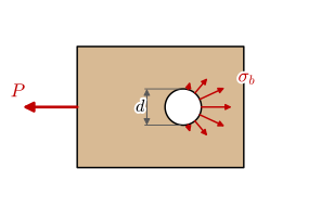
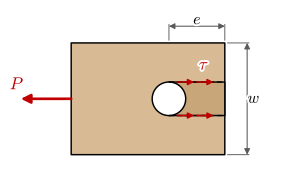
The pin presses on the half of the hole toward the plate end, Figure 8.4.12 (c). The contact pressure varies around the hole, and its average over the projected area \(dt\), the rectangle the pin covers when seen along the load, is the bearing stress. The same push drives the material between the hole and the plate end out of the plate, Figure 8.4.12 (d), by shearing it along two planes of length \(e - d/2\) each,
Finally the pin itself is cut at the one plane between the plates, in single shear like the pin at \(B\) in Figure 8.4.10, \(\tau_{\text{pin}} = P/(\pi d^2/4)\).
Code
P, w, t, d, e = sp.symbols('P w t d e', positive=True)K_t =3-3.14*(d/w) +3.667*(d/w)**2-1.527*(d/w)**3# Pilkey (2005)stresses = {r"\sigma_{\text{gross}}": P/(w*t),r"\sigma_{\text{net}}": P/((w - d)*t),r"\sigma_{\max}": K_t*P/((w - d)*t),r"\sigma_b": P/(d*t),r"\tau_{\text{out}}": P/(2*(e - d/2)*t),r"\tau_{\text{pin}}": P/(sp.pi*d**2/4)}values = {P: 20e3, w: 40, t: 5, d: 12, e: 20} # N and mm, so stresses in MPasigma_y_plate, sigma_y_pin =355, 640# shear yields at half the tensile yield stress, a conservative estimatelimits = {r"\sigma_{\text{gross}}": sigma_y_plate, r"\sigma_{\text{net}}": sigma_y_plate,r"\sigma_{\max}": sigma_y_plate, r"\sigma_b": sigma_y_plate,r"\tau_{\text{out}}": sigma_y_plate/2, r"\tau_{\text{pin}}": sigma_y_pin/2}rows = []for name, expr in stresses.items(): value =float(expr.subs(values)) rows += [(""ifnot rows elser"\\ ") + name +" &=", sp.Float(value),r"~\text{MPa}, \qquad \eta =", sp.Float(limits[name]/value)]ltx(*rows, aligned=True, precision=4)
The shear limits in the code take a material to yield in shear at half its tensile yield stress. That is a conservative estimate, and Chapter 8.7 shows where it comes from. The factor of safety of each mode is then its limit over its stress, as in 8.3.3.
The two lowest factors of safety are almost equal, \(\eta = 1.06\) for the peak stress at the hole edge and \(\eta = 1.07\) in bearing, and they mean different things. The peak stress is reached only in a thin band of material at the edge of the hole. In a ductile steel under a static load that band yields a little, the stress spreads over the rest of the net section, and the joint carries on; the net section itself has a factor of safety of \(2.5\). The peak matters when the load varies over time, because fatigue cracks start where the stress is highest, and in brittle materials, which cannot redistribute it. The bearing stress, in contrast, is an average over the whole contact, and exceeding it crushes the edge of the hole and lets the pin move, so under a static load bearing is what limits this joint. Design codes allow a bearing stress somewhat above \(\sigma_y\), because the material around the contact is confined, so comparing with \(\sigma_y\) as we did errs on the safe side.
Each mode points to its own remedy. A thicker plate lowers every plate stress at once. A larger edge distance \(e\) helps only tear-out, a wider plate only the tension modes, and a larger pin lowers the bearing and pin stresses but removes more of the net section. Designing a joint means balancing these against each other until no single mode is much weaker than the rest.
A lap joint has one more weakness that none of these formulas contains. The two plates do not lie in one plane, so the forces \(P\) are offset by the thickness \(t\) and form a couple that bends the plates and the pin. A double-shear joint, with one plate held between two others as in Example 1, is symmetric and avoids it.
Computing the stress concentration
The notebook below solves the plate of Figure 8.4.13 with the finite element method, for any width, hole, thickness, load and material. It meshes a quarter of the plate with six-node triangles, uses the two symmetry lines through the hole, and compares the computed \(K_t\) with the chart. Refining the mesh along the hole brings the two together.