12.2  Torsion of a round bar in Gridap

Hand solution

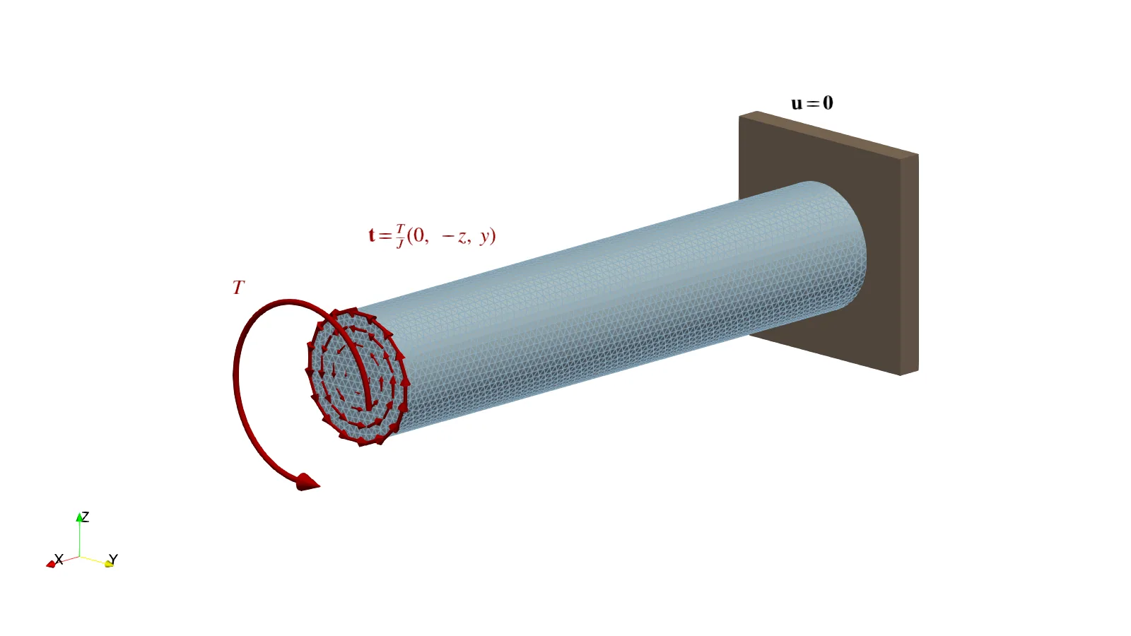
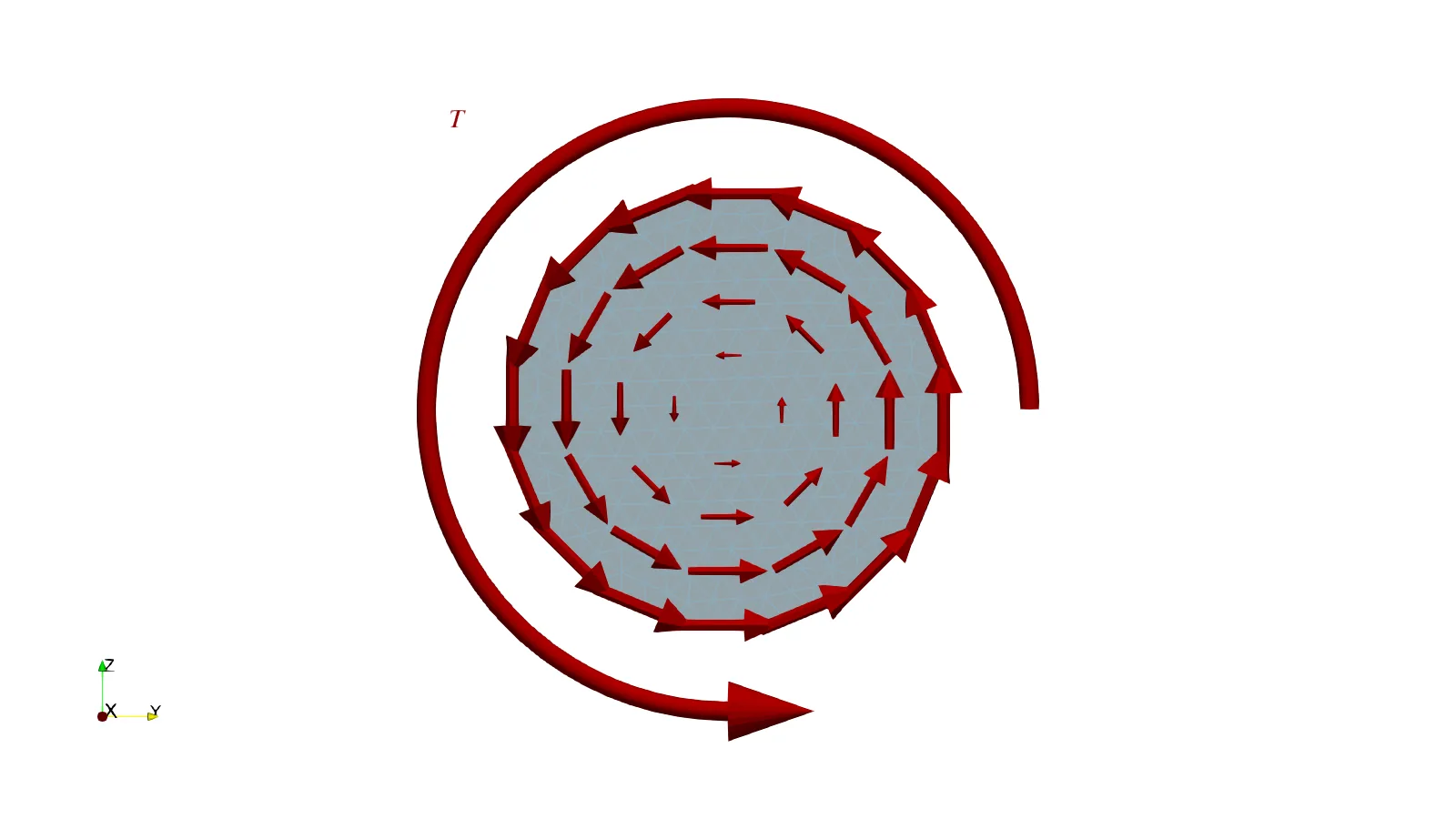
The polar moment of the solid section is \(J = \pi R^4/2\) and the shear modulus is \(G = E/(2(1+\nu))\). The shear stress grows linearly from zero on the axis to its largest value at the surface, and the twist angle grows linearly from the wall,

\[ \tau(r) = \frac{T r}{J}, \qquad \theta(x) = \frac{T x}{G J}. \tag{12.2.1}\]

R, L = 10.0, 100.0           # radius and length [mm]
E, nu = 210e3, 0.3           # steel [MPa]
T = 100e3                    # torque 100 Nm in Nmm

G = E/(2*(1 + nu))
J = float(sp.pi)*R**4/2
tau_max = T*R/J
theta_L = T*L/(G*J)

With the numbers of the example, the hand solution gives

The model as virtual work

The finite element model is the principle of virtual work for the whole bar. For every virtual displacement \(\delta\bm u\) that vanishes on the clamped end, the internal virtual work of the stresses equals the external virtual work of the traction \(\bm t\) on the loaded end,

\[ \int_\Omega \bm\sigma(\bm u) : \bm\varepsilon(\delta\bm u)\,d\Omega = \int_{\Gamma_L} \bm t \cdot \delta\bm u\,d\Gamma , \qquad \bm\sigma = \lambda\,\mathrm{tr}(\bm\varepsilon)\,\bm I + 2G\,\bm\varepsilon , \tag{12.2.2}\]

where \(\lambda = E\nu/((1+\nu)(1-2\nu))\) is Lamé’s first parameter. The clamp needs no term of its own: \(\delta\bm u = \bm 0\) there, so its reactions do no virtual work.

A torque is a resultant, and a three-dimensional model needs to know how it is spread over the end face. We spread it the way the exact solution does. In the torsion chapter the displacement of a circular shaft is \(\bm u = \theta(x)\,(0,\,-z,\,y)\), which gives the shear stresses \(\sigma_{xy} = -G\theta' z\) and \(\sigma_{xz} = G\theta' y\). On the end face, with outward normal \(\bm e_x\), the traction is the first row of \(\bm\sigma\), and with \(G\theta' = T/J\)

\[ \bm t = \bm\sigma\,\bm e_x = \frac{T}{J}\begin{bmatrix} 0 \\ -z \\ y \end{bmatrix}. \tag{12.2.3}\]

Its moment about the \(x\) axis is the applied torque and its force resultant is zero, as we check by integrating over the section in polar coordinates \(y = \rho\cos\varphi\), \(z = \rho\sin\varphi\):

rho, phi = sp.symbols('rho varphi', nonnegative=True)
T_s, J_s, R_s = sp.symbols('T J R', positive=True)
y_s, z_s = rho*sp.cos(phi), rho*sp.sin(phi)
t_y, t_z = -T_s/J_s*z_s, T_s/J_s*y_s

def over_section(f):
    return sp.integrate(sp.integrate(f*rho, (rho, 0, R_s)), (phi, 0, 2*sp.pi))

M_x = sp.simplify(over_section(y_s*t_z - z_s*t_y).subs(J_s, sp.pi*R_s**4/2))
F_y, F_z = over_section(t_y), over_section(t_z)

The clamp agrees with the exact solution as well. A circular section does not warp, so the exact displacement is zero over the whole face \(x = 0\), and clamping that face changes nothing. Both ends of the model therefore carry exactly the boundary conditions of the textbook solution, and 12.2.1 should hold everywhere in the bar, including next to the wall. For a square shaft the clamp would stop the section from warping, and the stresses near the wall would differ from Saint-Venant’s solution.

The Gridap model

The script Gridap/torsion/torsion.jl builds the geometry and the mesh with gmsh’s Julia interface. The cylinder’s two end faces are found by their centres of mass and named, because Gridap refers to boundaries by these names:

gmsh.initialize()
gmsh.model.add("bar")
vol = gmsh.model.occ.addCylinder(0, 0, 0, L, 0, 0, R)
gmsh.model.occ.synchronize()
faces = [t for (d, t) in gmsh.model.getBoundary([(3, vol)], false, false, false)]
xc(t) = gmsh.model.occ.getCenterOfMass(2, t)[1]
gmsh.model.addPhysicalGroup(2, [t for t in faces if isapprox(xc(t), 0, atol=1e-6)], -1, "fixed")
gmsh.model.addPhysicalGroup(2, [t for t in faces if isapprox(xc(t), L, atol=1e-6)], -1, "loaded")
gmsh.model.addPhysicalGroup(3, [vol], -1, "bar")
gmsh.option.setNumber("Mesh.MeshSizeMax", 2.5)
gmsh.option.setNumber("Mesh.MeshSizeFromCurvature", 48)
gmsh.model.mesh.generate(3)
gmsh.write("bar.msh")
gmsh.finalize()

The element size is 2.5 mm, and the curvature option puts 48 element edges around the circumference. Gridap then reads the mesh and sets up the function spaces. The test space V holds the virtual displacements, quadratic on each tetrahedron and zero on "fixed"; the trial space U holds the displacements, with the prescribed value zero on the same face. dΩ and dΓ are the integration rules over the volume and over the loaded face:

model = GmshDiscreteModel("bar.msh")
V = TestFESpace(model, ReferenceFE(lagrangian, VectorValue{3,Float64}, 2);
                conformity=:H1, dirichlet_tags=["fixed"])
U = TrialFESpace(V, VectorValue(0.0, 0.0, 0.0))
Ω = Triangulation(model); dΩ = Measure(Ω, 4)
Γ = BoundaryTriangulation(model, tags="loaded"); dΓ = Measure(Γ, 4)

The weak form 12.2.2 and the traction 12.2.3 are written almost as on paper, with v in the place of \(\delta\bm u\). AffineFEOperator assembles the stiffness matrix and the load vector, and solve returns the displacement field:

λ = E*ν/((1 + ν)*(1 - 2ν))
σ(ε) = λ*tr(ε)*one(ε) + 2G*ε
t(x) = (T/J)*VectorValue(0.0, -x[3], x[2])

a(u, v) = ∫(ε(v) ⊙ (σ∘ε(u)))dΩ
l(v) = ∫(v ⋅ t)dΓ
uh = solve(AffineFEOperator(a, l, U, V))

From the displacement we form the stress and the shear stress magnitude \(\tau = \sqrt{\sigma_{xy}^2 + \sigma_{xz}^2}\), and write all three to a VTU file for ParaView:

σh = σ∘ε(uh)
τh = (s -> sqrt(s[1,2]^2 + s[1,3]^2))∘σh
writevtk(Ω, "bar", cellfields=["u" => uh, "tau" => τh, "sigma" => σh])

The script finally samples \(\tau\) along the radius at mid-length and the twist \(\theta = u_z/y\) along the bar, and stores both as CSV files for the comparison below. The images are made from the VTU file by render.py and render_bc.py in the same folder, which run in ParaView’s pvbatch without opening a window. The cell below reruns the scripts only when their results are missing; the Julia solve takes about two and a half minutes on four cores.

here = Path('torsion')
if not (here/'summary.csv').exists():
    subprocess.run(['julia', 'torsion.jl'], cwd=here, check=True, capture_output=True)
for script, image in [('render.py', 'GridapTorsion_bar_end.png'),
                      ('render_bc.py', 'GridapTorsion_bar_bc.png')]:
    if not (Path('graphics')/image).exists():
        subprocess.run(['pvbatch', script], cwd=here, check=True, capture_output=True)

summary = dict(np.genfromtxt(here/'summary.csv', delimiter=',', dtype=None, encoding=None))
r_fe, tau_fe = np.loadtxt(here/'tau_r.csv', delimiter=',').T
x_fe, theta_fe = np.loadtxt(here/'theta_x.csv', delimiter=',').T

The mesh has the following size:

Results

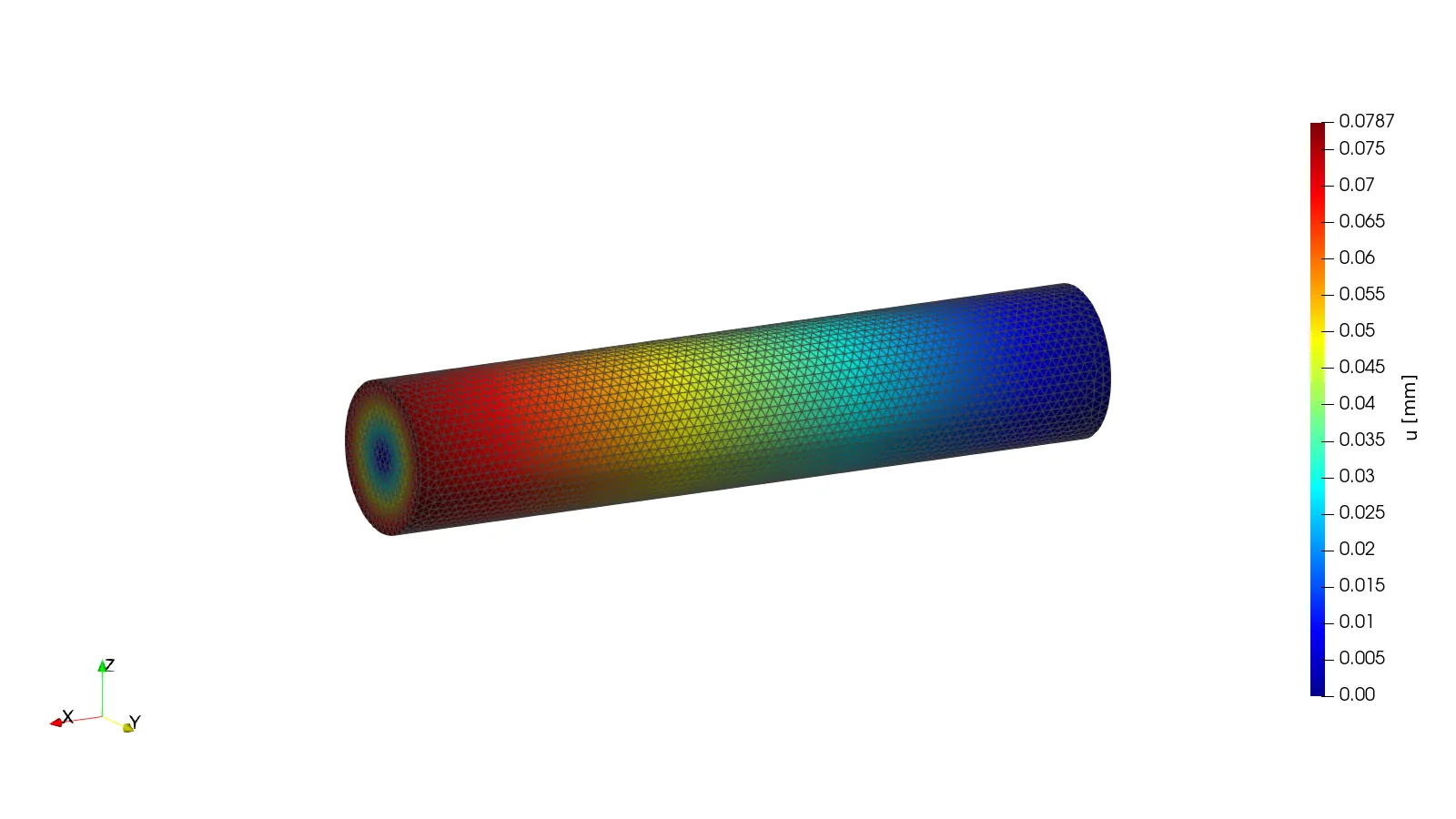
The displacement in Figure 12.2.2 grows linearly along the bar from zero at the wall, and on the end face it grows linearly with the distance from the axis, as \(|\bm u| = r\,\theta(x)\) requires. The largest displacement, at the surface of the free end, is \(R\,\theta(L) \approx 0.079\) mm.

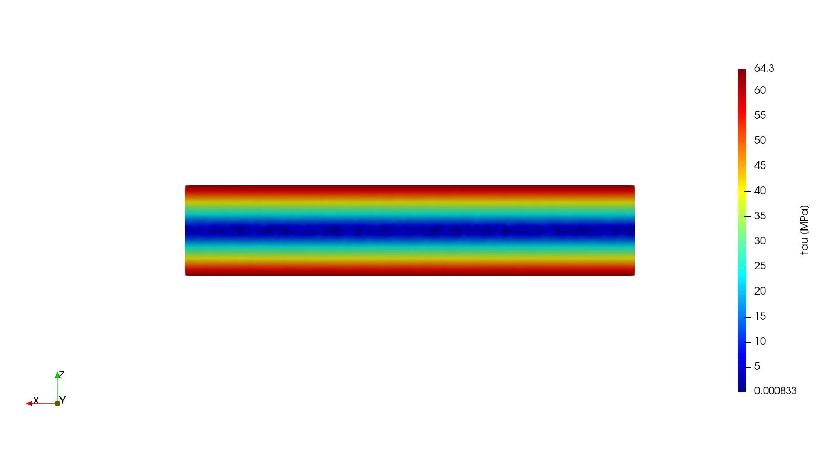
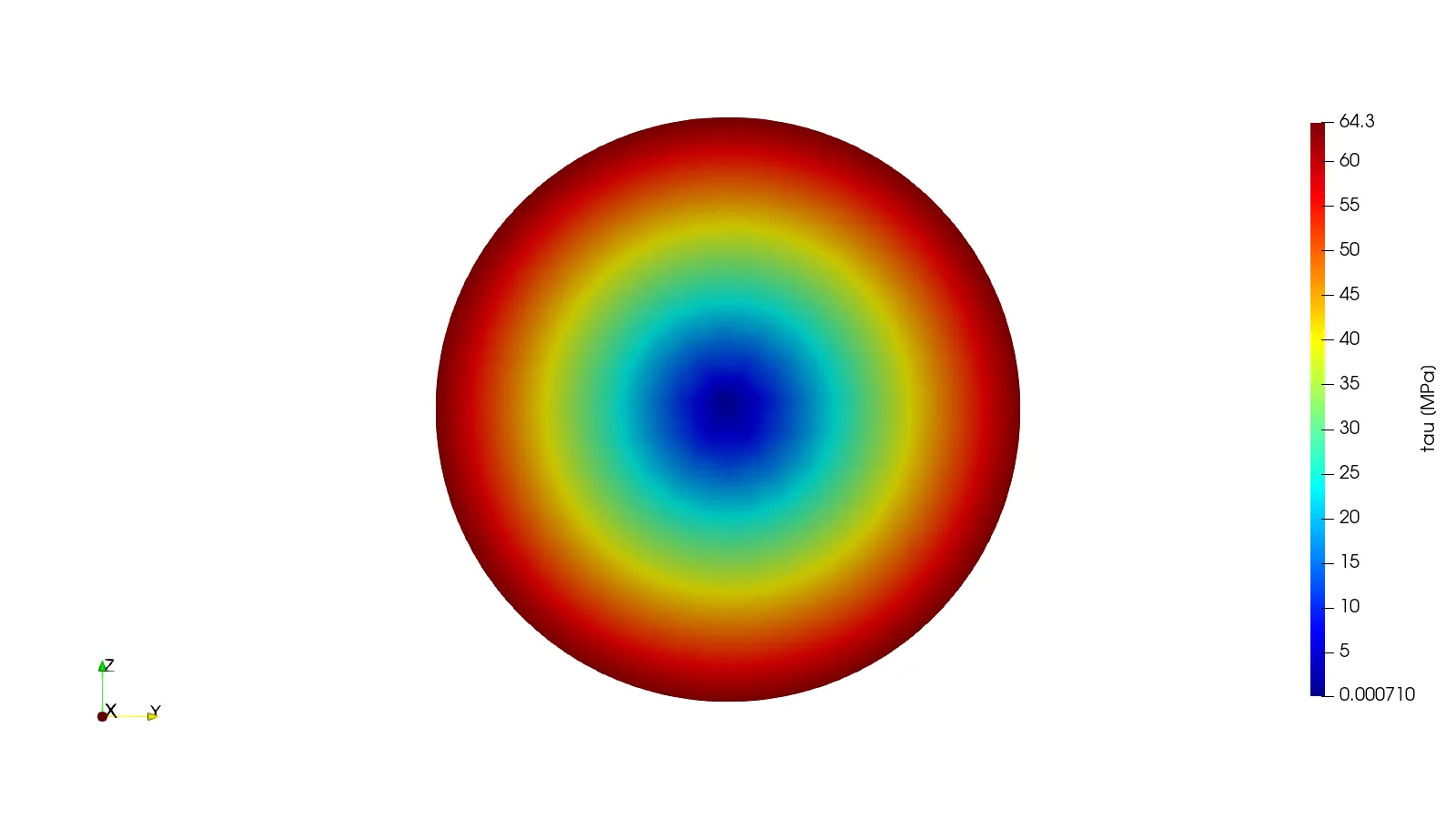
The shear stress is easier to read inside the bar. Figure 12.2.3 shows it on the cut through the axis: zero along the axis, largest at the surface, and the same at every \(x\), also next to the wall on the right. On the end face in Figure 12.2.4 the contours are circles, so \(\tau\) depends on \(r\) alone.

Comparison with the hand solution

The finite element value of \(\tau_{\max}\) is the stress at \(r = 0.995R\) on the line \(y\) through the middle of the bar, scaled to \(r = R\), and \(\theta(L)\) is \(u_z/y\) at \(y = 0.9R\) on the loaded end. Next to the hand values they give

The two differences are below 0.2 %. Figure 12.2.5 compares the whole profiles, the shear stress along the radius at mid-length and the twist angle along the bar, and the finite element points lie on the lines of 12.2.1.

fig, (ax1, ax2) = plt.subplots(1, 2, figsize=(9, 3.5))

r = np.linspace(0, R, 50)
ax1.plot(r, T*r/J, 'k-', label=r'hand, $Tr/J$')
ax1.plot(r_fe, tau_fe, 'o', ms=4, mfc='none', color='tab:blue', label='Gridap')
ax1.set(xlabel=r'$r$ [mm]', ylabel=r'$\tau$ [MPa]', xlim=(0, R), ylim=(0, None),
        xticks=[0, 2.5, 5, 7.5, R], yticks=[0, 20, 40, round(tau_max, 1)])
ax1.legend(frameon=False)

x = np.linspace(0, L, 50)
ax2.plot(x, np.degrees(T*x/(G*J)), 'k-', label=r'hand, $Tx/(GJ)$')
ax2.plot(x_fe, np.degrees(theta_fe), 'o', ms=4, mfc='none', color='tab:blue', label='Gridap')
ax2.set(xlabel=r'$x$ [mm]', ylabel=r'$\theta$ [deg]', xlim=(0, L), ylim=(0, None),
        xticks=[0, 25, 50, 75, L], yticks=[0, 0.1, 0.2, 0.3, round(np.degrees(theta_L), 3)])
ax2.legend(frameon=False)
fig.tight_layout()
plt.show()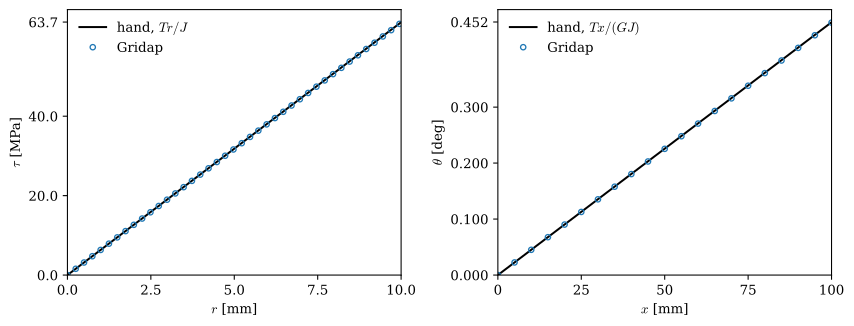

The small remaining difference has two sources. The mesh replaces the circle by 48 straight edges, so the meshed section is slightly smaller than the true one. The traction 12.2.3 is written with the exact \(J\) and integrated over the smaller section, so the applied torque and the stiffness of the bar shrink by nearly the same factor, and the stress and the twist barely notice. What remains is the error of quadratic tetrahedra of size 2.5 mm, and it shrinks when the mesh is refined.

The colour bars in Figure 12.2.3 and Figure 12.2.4 end at 64.3 MPa, above the hand value of 63.7 MPa. The stress in a quadratic element varies linearly, and ParaView shows it at the element corners, where the linear variation is extrapolated to the surface and overshoots slightly. The values in the comparison are taken inside the elements. The maximum of a colour bar is the least reliable number in a finite element result, and a stress read off at a surface should be checked against values just inside it.