“Ut tensio, sic vis; That is, The Power of any Spring is in the same proportion with the Tension thereof.”
— Robert Hooke, Lectures de Potentia Restitutiva, or of Spring, 1678
A spring is a part designed to deform. Every other machine element in this book is judged by how little it moves under load, whereas a spring is judged by how much it moves and by how predictably the force follows the motion. It turns a displacement into a force and a force into a displacement, and it stores the work done on it as elastic energy that it can give back almost without loss.
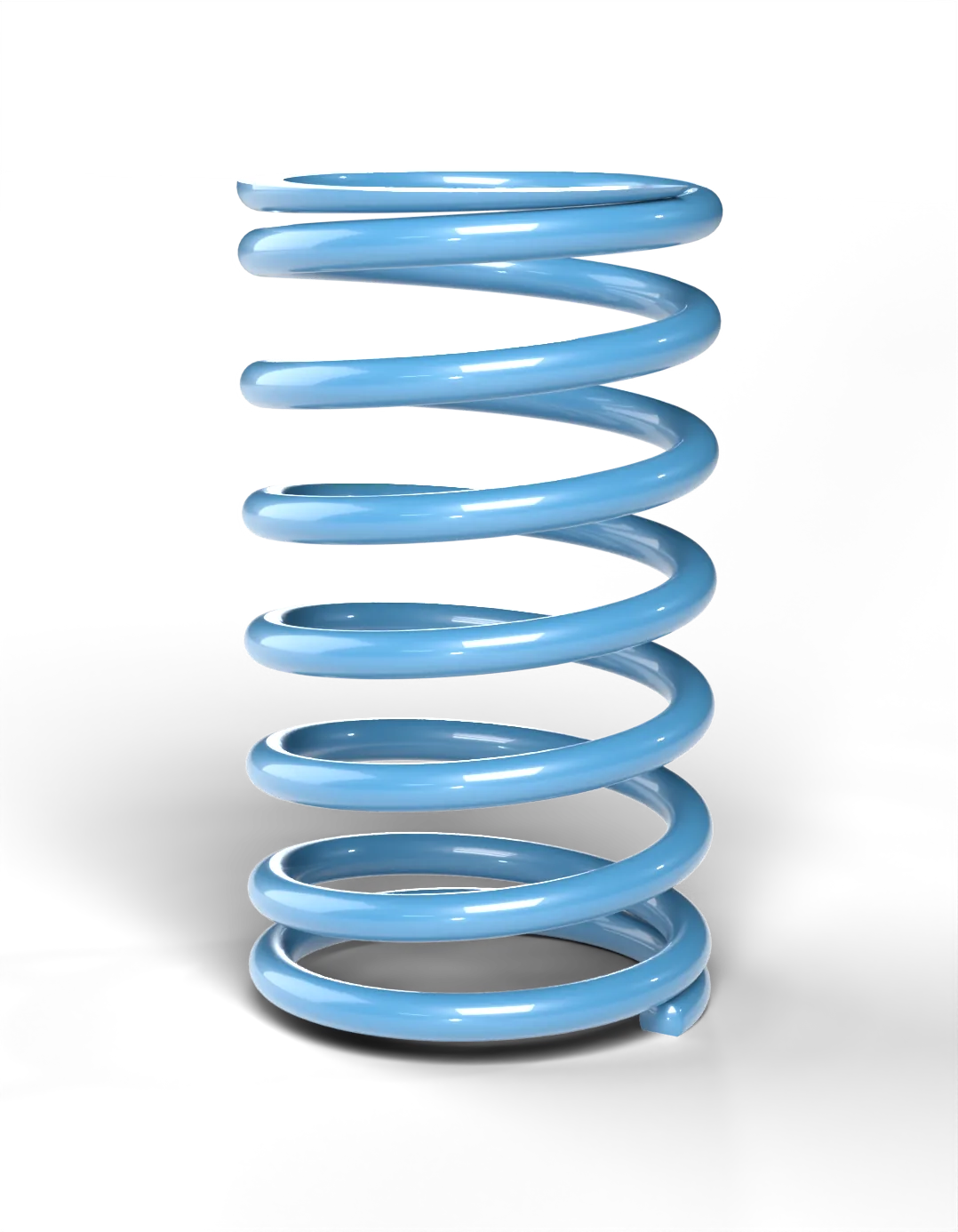
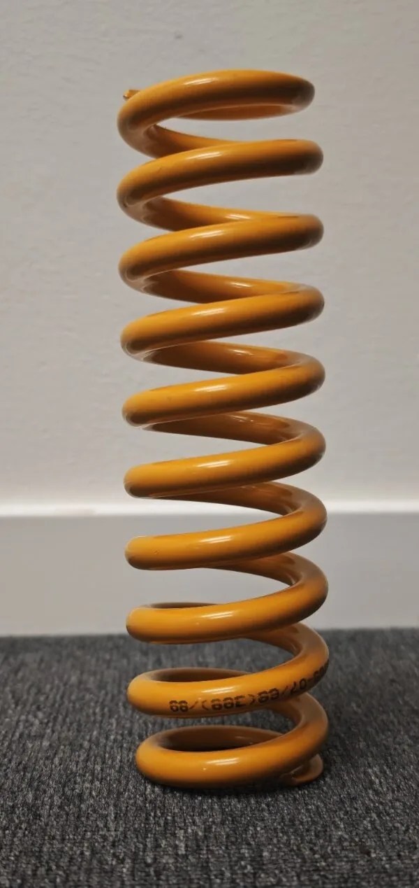
Figure 9.8.1: A helical compression spring with closed and ground ends.
We begin with what springs are used for and with the curve that describes any spring, the force against the deflection. Combining springs in series and in parallel follows directly from that curve. The helical compression spring then gets a full treatment: its rate follows from the torsion of a straight bar, the stress needs a correction for the curvature of the wire, its length invites buckling, and a caliper and a kitchen scale are enough to measure an unknown one. Torsion springs, extension springs and the other common types follow, and the chapter closes with what changes when a spring is printed.
What springs are for
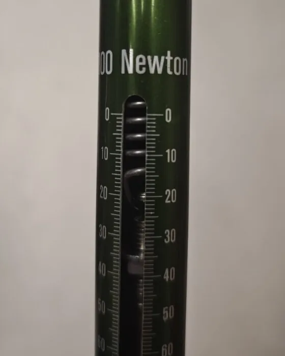
A spring can measure a force. One of known rate deflects in proportion to the load, so reading the deflection reads the force. The spring scale in Figure 9.8.2 (a) is the plainest example, and a strain-gauge load cell works on this principle with a far stiffer spring and an electrical reading of a far smaller deflection.
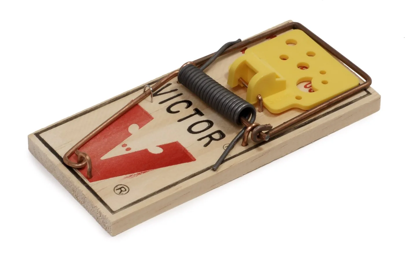
A spring can also generate a force. The mousetrap in Figure 9.8.2 (b) holds a torsion spring wound up, ready to deliver its moment the moment the catch is released. Valve springs, the clips that hold a battery and the spring that returns a pedal all do this: they hold a part against a seat or return it there.
(a) Measuring a force
(b) Generating a force
(c) Storing energy
(d) Absorbing shocks
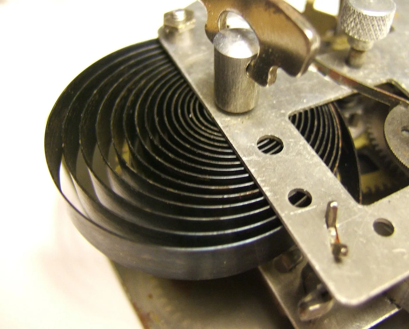
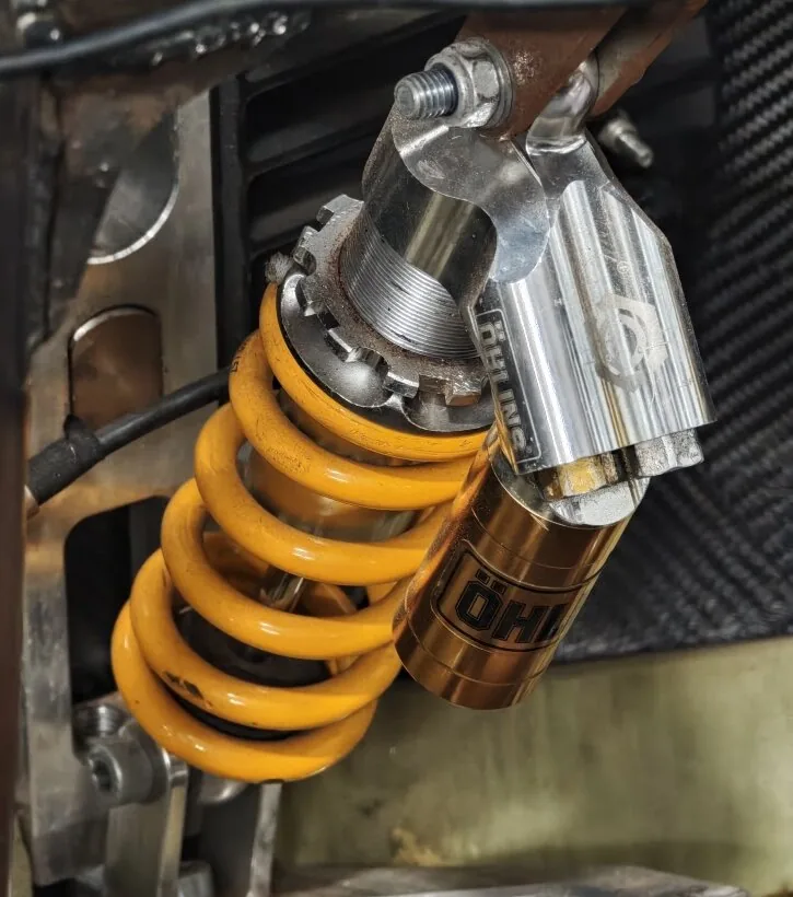
Figure 9.8.2: Four jobs for a spring. (a) A spring scale for up to \(100\) N. The end of the helical spring inside the tube shows through the slot against the scale. (b) A snap mousetrap, driven by a wound torsion spring. (c) The spiral mainspring of an alarm clock. (d) The coil-over unit of the front left suspension of the Jönköping Solar Team car, a coil spring around a damper.
Springs store energy and release it at a controlled rate. The mainspring in Figure 9.8.2 (c) is a long strip wound into a spiral, and the clock draws its energy back one escapement tick at a time. A drawn bow releases its energy all at once.
Finally, springs cope with dynamic loads. The coil spring of a vehicle suspension, Figure 9.8.2 (d), lets the wheel follow the road while the frame moves far less, and the damper inside it removes the energy that would otherwise keep the spring oscillating. Springs under machines isolate vibration: a soft spring carrying a heavy mass has a low natural frequency, and excitation well above that frequency is barely transmitted.
The spring characteristic
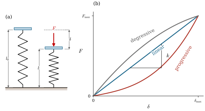
Whatever its shape, a spring is described by its characteristic, the force \(F\) needed to hold it at a deflection \(\delta\). For the compression spring of Figure 9.8.3 (a) the deflection is the shortening from the free length \(l_0\) to the loaded length \(l\), \(\delta = l_0 - l\). The slope of the characteristic is the spring rate, or stiffness,
\[
k = \frac{dF}{d\delta}
\tag{9.8.1}\]
and when the characteristic is a straight line through the origin, the rate is constant and we recover Hooke’s law,
\[
F = k\delta
\tag{9.8.2}\]
The work done on the spring is the area under the characteristic. A linear spring loaded from zero to \(\delta\) stores
\[
U = \int_0^\delta F\,d\delta = \frac{1}{2}k\delta^2 = \frac{1}{2}F\delta
\tag{9.8.3}\]
and returns it on unloading, apart from a small loss to friction and material damping.
Figure 9.8.3: (a) A compression spring unloaded, at its free length \(l_0\), and loaded by \(F\) to the length \(l\). (b) Linear, progressive and degressive characteristics. The slope of the line is the rate \(k\).
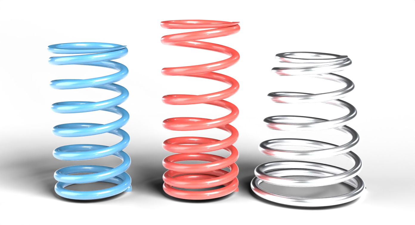
A progressive characteristic stiffens with deflection and a degressive one softens. Both are designed in on purpose. A vehicle spring is often made progressive so that it is soft for small bumps and stiff enough not to bottom out on large ones. Two ways of achieving it with a helical spring are shown in Figure 9.8.4. When the pitch varies along the spring, the closely spaced coils close up first, and every coil that touches its neighbour stops contributing, so the remaining spring has fewer active coils and a higher rate. A conical spring is progressive too, because its large coils are softer and bottom out first. A degressive characteristic is typical of disc springs, which can be proportioned to give an almost constant force over part of their stroke.
Figure 9.8.4: Three compression springs: constant pitch, which is linear, variable pitch, and conical. The last two are progressive.
Springs in series and in parallel
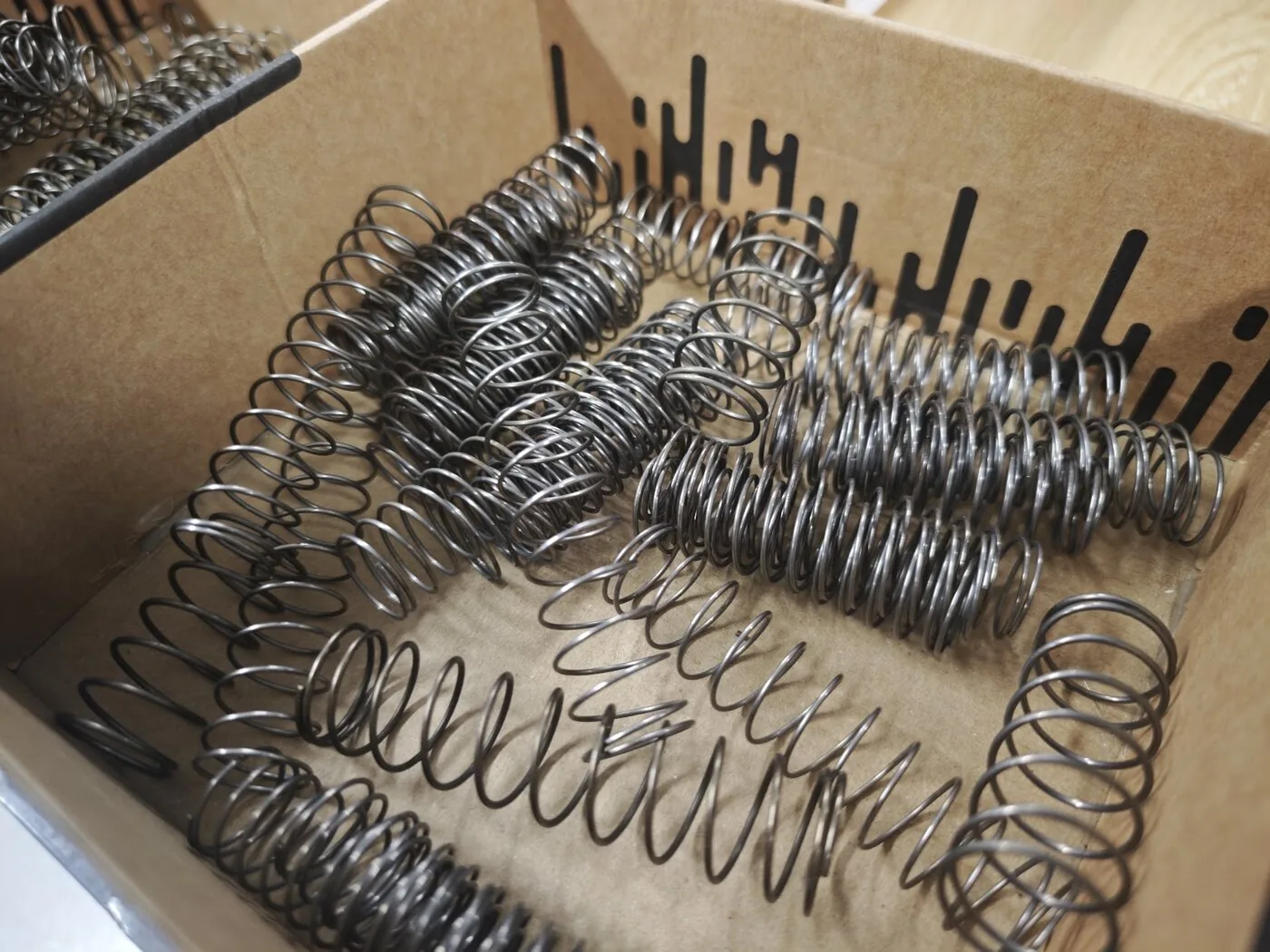
Springs are often combined, either to reach a rate that no single available spring has, or to shape a characteristic. A stock of springs such as Figure 9.8.5 seldom holds the exact rate a design asks for, but two of them together often come close. The two basic arrangements are shown in Figure 9.8.6.
Figure 9.8.5: A box of compression springs. Each has its own wire diameter, coil diameter and number of coils, and so its own rate.
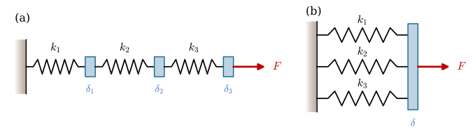
Figure 9.8.6: Three springs (a) in series, where each carries the whole force and the deflections add, and (b) in parallel, where each sees the whole deflection and the forces add.
In parallel every spring is deflected by the same \(\delta\), so spring \(i\) carries \(F_i = k_i\delta\), and equilibrium of the rigid bar requires the forces to add up to the load, \(F = \sum_i k_i\delta\). The combined rate is therefore the sum of the rates,
\[
k = \sum_{i=1}^{n} k_i
\tag{9.8.4}\]
In series the same force passes through every spring, which follows from the equilibrium of each of the small blocks between them. Spring \(i\) then deflects by \(\delta_i = F/k_i\), and the deflections add up to the total, \(\delta = \sum_i F/k_i\). It is now the flexibilities\(1/k_i\) that add,
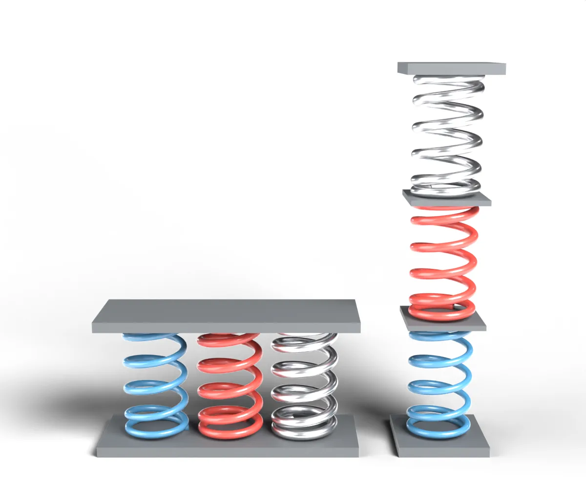
Two consequences are useful to keep in mind. A parallel group is always stiffer than its stiffest member, and a series chain is always softer than its softest member. And in a series chain the deflection is shared in inverse proportion to the rates, \(\delta_i/\delta = k/k_i\), so the softest spring takes the largest share of the stroke and is the first to close up. Figure 9.8.7 shows both arrangements built from one set of three springs and compressed by equal displacements. In the series stack the soft blue spring visibly does most of the moving, and the graph shows the parallel group needing about twelve times the force of the series chain.
Figure 9.8.7: Three springs in parallel and in series, both compressed by up to \(12\) mm. The dashed lines are the characteristics of the single springs, and the solid lines are those of the two combinations, with the slopes of 9.8.4 and 9.8.5. The numbers are worked out in Example 2.
The helical compression spring
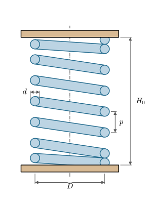
The helical compression spring is a wire of diameter \(d\) wound into a helix of mean coil diameter \(D\), Figure 9.8.8. Of its coils, \(n\) are active and deflect under load. The end coils of a spring that is to sit squarely on a flat seat are closed, wound at a pitch equal to the wire diameter so that they touch, and usually also ground flat. They carry the load into the seat but do not deflect, so a spring with closed ends has \(n_t = n + 2\) coils in total. The active coils advance by the pitch \(p\) per turn, and the spring has the free height \(H_0\) when unloaded. The ratio
\[
C = \frac{D}{d}
\tag{9.8.6}\]
is the spring index. Springs are normally wound with \(C\) between about \(4\) and \(12\). Below that the wire is bent so sharply in winding that it cracks, and above it the spring is floppy and tangles [1].
(a) As a part.
(b) As an engineering drawing shows it.
Figure 9.8.8: A helical compression spring with closed and ground ends. The ground ends sit flat on the two seats.
The wire is twisted, not bent
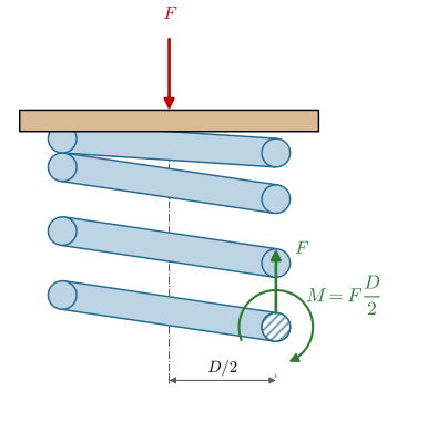
A compression spring looks as though it should behave like a stack of bent rings, but the wire is in fact loaded in torsion. We see this by cutting the spring with a plane through its axis and drawing the free body of the upper part, Figure 9.8.9. The load \(F\) acts along the axis of the spring, while the cut exposes a cross section of the wire at the distance \(D/2\) from that axis. Equilibrium of forces requires a shear force \(F\) on the section, and equilibrium of moments about the centre of the section requires a moment
\[
M = F\frac{D}{2}
\tag{9.8.7}\]
At this cut the wire runs perpendicular to the drawing, so \(M\) acts about the axis of the wire: it is a torque. The argument holds at every cut, because a spring loaded along its axis looks alike from every angle, so the whole length of wire carries the constant torque of 9.8.7 plus the shear force \(F\). We have neglected the slope of the coils, the helix angle, which is small as long as the pitch is small compared with the circumference \(\pi D\).
Figure 9.8.9: The upper part of a compression spring, cut through its axis. The exposed wire section carries the shear force \(F\) and the torque \(M = FD/2\) about the axis of the wire.
The spring rate from the torsion of the wire
The wire can now be straightened out in our minds into a bar of length \(L = \pi D n\), the length of the active coils, twisted by the torque \(M\). The torsion chapter gives the angle of twist of such a bar, 8.13.7,
where \(G\) is the shear modulus of the wire and \(J\) the polar moment of area of its circular section. Each section of the wire turns in proportion to its distance \(s\) along the wire, \(\theta(s) = Ms/(GJ)\), so the end of the active wire turns by the whole \(\theta\), Figure 9.8.10. Consider a short piece of wire \(ds\). Its twist \(d\theta\) turns all of the spring beyond it rigidly about the axis of the wire at that point, and the load, which acts on the spring axis at the lever arm \(D/2\), moves along the axis by \((D/2)\,d\theta\). Adding up these contributions over the whole wire, the deflection is \(\delta = (D/2)\theta\), and with 9.8.7,
\[
\delta = \frac{D}{2}\,\frac{F(D/2)\,\pi D n}{G\,\pi d^4/32} = \frac{8FD^3n}{Gd^4}
\tag{9.8.8}\]
The deflection is proportional to the force, so the helical spring is linear with the rate
We let SymPy repeat the derivation, and then check it by a second route, the energy method.
Figure 9.8.10: The upper part of the spring of Figure 9.8.9 under a rising and falling load, with the cut section held still. The stripes are painted along the wire, and each section turns about the wire axis by \(\theta(s) = Ms/(GJ)\): hardly at all next to the cut, and most on the last active coil, where \(\theta = ML/(GJ)\). The coils close up and the plate moves down by \(\delta = (D/2)\theta\). The pitch is drawn larger than usual so that the twist can be seen.
Code
F, D, d, n, G = sp.symbols('F D d n G', positive=True)M = F*D/2# torque on every wire section, from the free bodyL = sp.pi*D*n # length of the active wireJ = sp.pi*d**4/32# polar moment of area of the wiretheta = M*L/(G*J) # angle of twist of the straightened wiredelta = theta*D/2# the load moves by the twist times its lever arm
SymPy returns the deflection and the rate,
\[ \delta =\dfrac{8 D^{3} F n}{G d^{4}},\qquad k = \frac{F}{\delta} =\dfrac{G d^{4}}{8 D^{3} n} \]
Code
U = M**2*L/(2*G*J) # strain energy of the twisted wiredelta_U = sp.diff(U, F) # Castigliano: the deflection at the load
The strain energy of a twisted bar is \(U = M^2L/(2GJ)\), and Castigliano’s theorem (Energy methods) gives the deflection at the load as \(\delta = \partial U/\partial F\). The difference between the two results vanishes, so the two routes agree.
9.8.9 tells the designer where the stiffness comes from. The rate grows with the fourth power of the wire diameter, so a wire \(40\,\%\) thicker gives a spring almost four times as stiff, which is the difference between the three springs of Figure 9.8.7. It falls with the cube of the coil diameter, and it is inversely proportional to the number of active coils, which is 9.8.5 in disguise: each coil is a spring in series with the others.
Stress in the wire
The torque produces the shear stress of 8.13.5, largest at the surface of the wire,
and the shear force \(F\) adds an average shear stress \(4F/(\pi d^2)\). On the inside of the coil, the side facing the spring axis, the two act in the same direction and add,
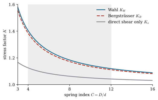
Curvature adds a second effect on the inside. The wire is curved, so a fibre on the inside of the coil is shorter than one on the outside, and a given twist strains it more. The analysis of a twisted curved bar is beyond our scope, but its result is a correction factor on the straight-bar stress that grows as the index falls. Two forms are in use, Wahl’s and Bergsträsser’s, and both include the direct shear [1,2],
with \(K = K_W\) or \(K_B\). The two agree within two percent, Figure 9.8.11, and the simpler \(K_B\) is the one we use. For a static load the stress may be checked against the torsional yield strength of the wire. Under fatigue loading the curvature factor matters even more, because cracks start on the inside of the coil, and the analysis follows the fatigue chapter.
Figure 9.8.11: Stress correction factors against the spring index. The shaded band is the usual range of \(C\). The gap between \(K_s\) and the other two is the effect of curvature.
Solid length and buckling
A compression spring cannot be shortened beyond the point where all its coils touch. With closed ends the solid length is close to \(L_s = n_t d\), and the largest possible deflection is \(H_0 - L_s\). A well designed spring survives being pressed solid, because sooner or later someone will do it, and Example 1 shows that this is a real constraint.
A long compression spring is also a slender column, and it can buckle sideways under its own axial load like the struts of the buckling chapter, Buckling. Its critical load depends on both the bending and the shear stiffness of the coil, and the classic analysis is Haringx’s [3]. According to [1], it shows that a spring cannot buckle at any deflection as long as its free height satisfies
where \(\alpha\) is the effective length factor of the end supports, defined as for a column. The material enters only through the ratio of its two moduli. With \(E = 2G(1 + \nu)\) the root becomes \(\sqrt{(1 + 2\nu)/(2 + \nu)}\), which is about \(0.84\) for steel, \(\nu \approx 0.3\), and the condition for steel springs is
\[
H_0 < 2.63\,\frac{D}{\alpha}
\tag{9.8.14}\]
A spring pressed between two flat, parallel plates that cannot tilt has \(\alpha = 0.5\) and is stable up to \(H_0 \approx 5.3D\). A spring whose ends can pivot has \(\alpha = 1\), and the limit falls to \(H_0 \approx 2.6D\), the conservative value often quoted on its own. Springs that are longer still are guided by a rod through their centre or a tube around them.
Example 1: Checking a compression spring
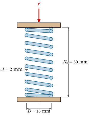
A compression spring with closed and ground ends is wound from hard-drawn spring steel wire of diameter \(d = 2\) mm, with a mean coil diameter \(D = 16\) mm, \(n = 8\) active coils and a free height \(H_0 = 50\) mm, Figure 9.8.12. The shear modulus is \(G = 79.3\) GPa. In service the spring is compressed by \(\delta = 10\) mm between two parallel plates. We find the rate, the force, the largest shear stress, and check what happens if the spring is pressed solid and whether it can buckle.
Figure 9.8.12: Example 1. A compression spring between two flat plates, with \(n = 8\) active coils.
The rate follows from 9.8.9 and the force from Hooke’s law. With the index \(C = 16/2 = 8\), the Bergsträsser factor of 9.8.11 gives the largest stress through 9.8.12.
Code
k = sp.simplify(F/delta) # @eq-spring-rate-helicalK_B = (4*D/d +2)/(4*D/d -3) # @eq-spring-wahl with C = D/dtau_max = K_B*8*F*D/(sp.pi*d**3) # @eq-spring-stressex1 = {G: 79.3e3, d: 2, D: 16, n: 8} # N/mm^2 and mmex1[F] = k.subs(ex1)*10# compressed by delta = 10 mm
To judge the stress we need a strength. The tensile strength of hard-drawn spring wire depends on its diameter, because thinner wire is drawn harder, and Shigley tabulates it as \(S_{ut} = A/d^m\) with \(A = 1783\) MPa\(\cdot\)mm\(^m\) and \(m = 0.190\) for \(d\) in mm. Shigley also recommends a torsional yield strength of \(S_{sy} = 0.45\,S_{ut}\) for static loading of this wire [1]. Pressed solid, the spring is \(n_t d = 10 \cdot 2 = 20\) mm high and has deflected by \(30\) mm.
Code
H_0 = sp.symbols('H_0', positive=True)S_ut =1783/d**sp.Rational(19, 100) # hard-drawn wire, MPa with d in mmS_sy = sp.Rational(45, 100)*S_utL_s = (n +2)*d # solid length with closed endsF_solid = k*(H_0 - L_s)delta_allow = S_sy/(tau_max/F)/k # deflection at which tau_max reaches S_syex1[H_0] =50
Pressed solid, and at the deflection where the stress reaches the yield strength,
In service the stress of about \(290\) MPa is well below the \(700\) MPa the wire tolerates. Pressed solid it would reach about \(870\) MPa and take a permanent set, so the spring is not solid safe: it can only be compressed by about \(24\) mm before it starts to yield. Either the installation must stop the stroke before that, or the spring needs fewer coils of thicker wire, or a stronger wire. Buckling is no concern. The ratio \(H_0/D = 50/16 = 3.1\) is above the pivoted-end limit of \(2.63\) but well below the limit of \(5.3\) for parallel plates, 9.8.14, and the plates in this installation are parallel.
The same check for any spring, with the wires of Shigley’s tables and the buckling condition 9.8.13 for every kind of seat, is in the configurator below. It opens on the spring of this example.
Example 2: Three springs in series and in parallel
Three springs are wound from one steel, \(G = 79.3\) GPa, with \(D = 17\) mm and \(n = 4\) active coils, and differ only in their wire diameters, \(d = 2.0\), \(2.4\) and \(2.8\) mm. They are mounted in parallel between two plates, and in series in a stack separated by thin plates, Figure 9.8.13. Both systems are compressed by \(\delta = 12\) mm. We find the rate of each spring and of each system, the force needed, and how the stroke is shared in the series stack.
Figure 9.8.13: Example 2. The three springs in parallel (left) and in series (right), unloaded.
Code
rate = sp.lambdify(d, k.subs({G: 79.3e3, D: 17, n: 4})) # @eq-spring-rate-helical, N/mmk_i = rate(np.array([2.0, 2.4, 2.8]))k_par = k_i.sum() # @eq-spring-parallelk_ser =1/np.sum(1/k_i) # @eq-spring-seriesdelta_i = k_ser*12.0/k_i # each series spring carries the same force
For the three springs and the two systems compressed by \(12\) mm,
The rates follow the fourth power of the wire diameter, roughly \(1 : 2 : 4\). The parallel group is stiffer than the stiffest spring and the series chain softer than the softest, and compressing the parallel group by \(12\) mm takes \(670\) N against \(56\) N for the chain. In the chain one force runs through all three springs, so the soft spring takes \(6.9\) mm of the stroke, more than half, and the stiff one only \(1.8\) mm. That is what Figure 9.8.7 shows.
Measuring a spring
A spring taken from a box such as Figure 9.8.5 comes without a data sheet, but a caliper and a kitchen scale find its rate and, with some care, its material. The geometry comes first. The caliper gives the wire diameter \(d\), best as the mean of a few readings round the wire, the outside diameter \(D_o\) and the free height \(H_0\). The mean coil diameter is the outside diameter less one wire diameter,
\[
D = D_o - d
\tag{9.8.15}\]
The total number of coils \(n_t\) is counted along the wire from one end to the other, and the ends decide how many of them are active. According to [1], closed ends, ground or not, leave \(n = n_t - 2\) active coils, open ends that are ground leave \(n = n_t - 1\), and plain open ends leave all of them active.
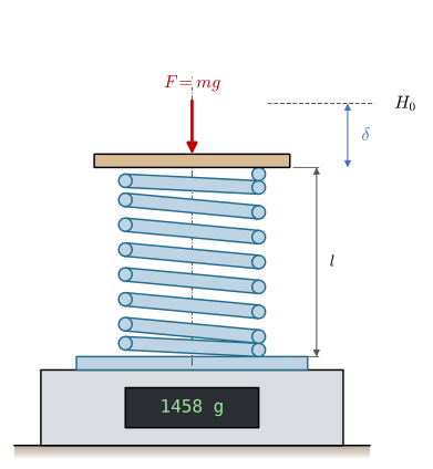
The rate comes from the scale, Figure 9.8.14. The spring stands on the pan, and the scale is zeroed with the spring on it, so that it reads the force on the top of the spring and nothing else. A flat plate on top compresses the spring to the length \(l\), which the caliper measures. The plate is best held still by a drill press or a screw clamp, since a hand cannot hold it steady while the caliper is read, and its weight is part of the force. Each reading \(m_j\) of the scale gives a force and a deflection,
The points follow the characteristic of Figure 9.8.3, but not exactly along a line through the origin. The ends seat themselves during the first millimetres, and every reading carries some error. We therefore fit the straight line \(F = F_0 + k\delta\) by least squares, choosing \(F_0\) and \(k\) so that the sum of the squared misfits \(\sum_j (F_j - F_0 - k\delta_j)^2\) is as small as possible. Setting its derivatives with respect to \(F_0\) and \(k\) to zero gives
where the bars are mean values over the \(N\) readings. The slope is the rate, and the intercept \(F_0\) only takes up the seating of the ends. Readings close to the solid length do not belong in the fit, because coils that touch stiffen the spring.
With the rate measured, 9.8.9 solved for the shear modulus gives
\[
G = \frac{8 D^3 n k}{d^4}
\tag{9.8.18}\]
which tells the material. According to the tables in [1], steel spring wires have \(G\) between about \(77\) and \(83\) GPa, the common stainless wires (302, 304 and 316) about \(69\) GPa and phosphor bronze about \(41\) GPa. The hardened stainless grades lie inside the steel range and cannot be told from steel this way. The fourth power of \(d\) makes the result sensitive to the caliper. For small errors the relative errors add, each weighted by its power in 9.8.18,
so a wire diameter read one percent wrong moves \(G\) by four percent, more than half the whole spread of the steel wires.
Example 3: Identifying a spring from the box
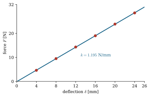
A spring from the box of Figure 9.8.5 has closed ends and \(n_t = 12\) coils. The caliper reads \(d = 1.20\) mm, \(D_o = 13.20\) mm and \(H_0 = 50.0\) mm, to within \(0.01\) mm for each reading. Pressed on a kitchen scale that reads to \(1\) g, Figure 9.8.14, the spring gives the readings of Table 9.8.1. We find the rate, the shear modulus and how sure we can be of the material.
Table 9.8.1: Example 3. Loaded length and scale reading.
\(l\) [mm]
\(46\)
\(42\)
\(38\)
\(34\)
\(30\)
\(26\)
\(m\) [g]
\(470\)
\(966\)
\(1458\)
\(1936\)
\(2431\)
\(2906\)
Figure 9.8.14: Example 3. The spring on the pan of a kitchen scale, pressed by a plate to the length \(l\), a deflection \(\delta\) below its free height \(H_0\).
By 9.8.15 the mean coil diameter is \(D = 13.20 - 1.20 = 12.00\) mm, and the closed ends leave \(n = 12 - 2 = 10\) active coils. 9.8.16 turns the readings into forces and deflections, 9.8.17 gives the rate and 9.8.18 the shear modulus. The scatter of the points about the line sets the uncertainty of the rate, through the standard error of the slope,
Figure 9.8.15: The six readings of Table 9.8.1 and the least-squares line through them.
The rate is \(1.195\) N/mm, known to a third of a percent, and the intercept of \(-0.1\) N is small, so the ends seated almost at once. The shear modulus of \(79.7\) GPa lies inside the steel range and far from the common stainless wires and from bronze, so the spring is of steel wire, or of one of the hardened stainless grades that share its modulus. Which steel it is the measurement cannot tell. The uncertainty of about four percent comes almost entirely from the wire diameter, which enters to the fourth power, and spans the whole range from oil-tempered wire to music wire. A micrometer that reads \(d\) to \(0.001\) mm would narrow it to about one percent.
The configurator below does the same with your own readings, typed or pasted one pair per line, and marks which of the tabled wires the measured modulus fits.
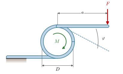
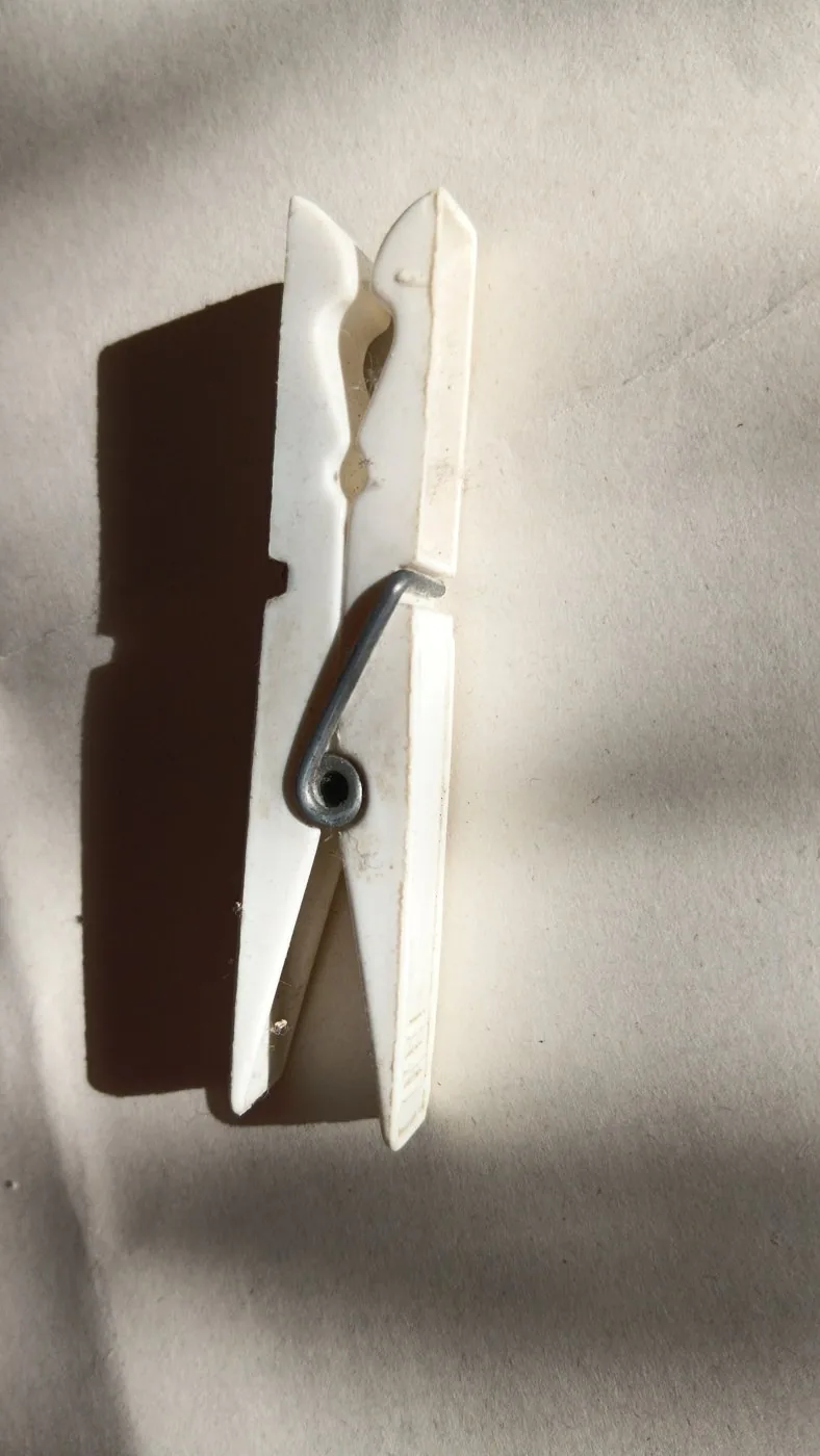
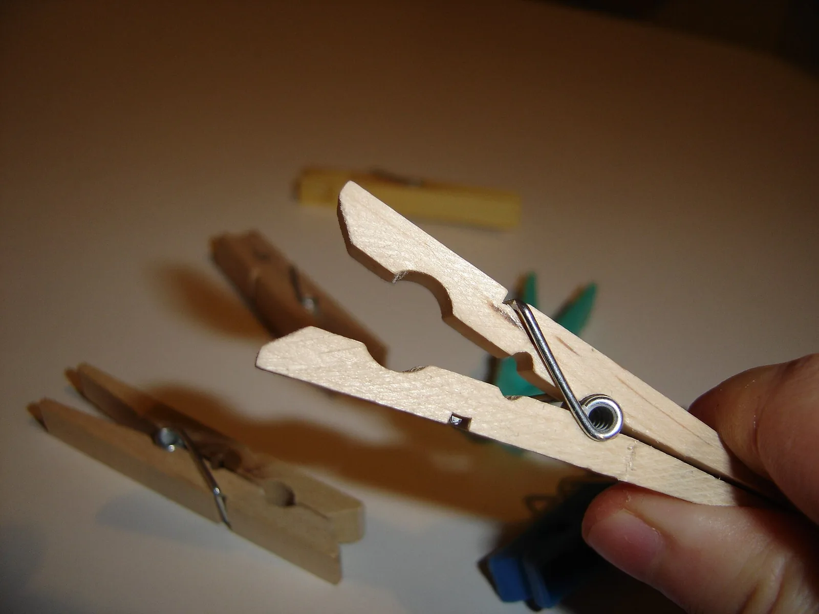
A helical torsion spring is wound like a compression spring, usually close wound, with the ends of the wire bent out into straight legs, Figure 9.8.16 (a). It is loaded by a moment about its own axis, applied through a force on a leg at the arm \(a\), \(M = Fa\). The clothes peg and the mousetrap of Figure 9.8.2 are the familiar examples, and Figure 9.8.16 (b) shows the first of them.
(a) A torsion spring loaded by \(F\) on one leg while the other leg rests on a stop. The leg turns through \(\varphi\) under the moment \(M = Fa\).
(b) The torsion spring of a clothes peg.
Figure 9.8.16: The helical torsion spring.
The roles of torsion and bending are now swapped. The moment acts about the coil axis, and at every section of the wire that axis is perpendicular to the wire, so the wire is bent by the constant moment \(M\). The wound coil turns through the angle of a bent bar of length \(L = \pi D n\). The moment-curvature relation 8.16.9 gives the change of slope \(d\varphi = M\,ds/(EI)\) along the wire, and integrating over its length,
\[
\varphi = \frac{ML}{EI}, \qquad I = \frac{\pi d^4}{64}
\]
which gives
\[
\varphi = \frac{64 M D n}{E d^4}, \qquad
\boxed{k = \frac{M}{\varphi} = \frac{E d^4}{64 D n}}
\tag{9.8.20}\]
with the rate now in moment per radian, and the elastic modulus \(E\) in place of \(G\). The legs bend as well and add a little to \(\varphi\), which 9.8.20 neglects. The bending stress is \(32M/(\pi d^3)\), corrected for curvature by the factor for the inside of the coil [1],
Winding the spring up reduces its coil diameter, so a torsion spring on an arbor needs clearance, and it should be loaded in the sense that winds it up, which puts the residual stress from coiling to good use.
Example 4: The clothes peg
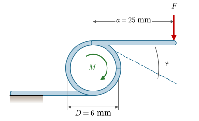
The spring of a clothes peg is modelled as a torsion spring of hard-drawn steel wire, with \(d = 1.5\) mm, \(D = 6\) mm, \(n = 2.5\) coils and \(E = 206\) GPa, Figure 9.8.17. With the peg fully open the legs have turned \(\varphi = 0.25\) rad from the free position, and the fingers press on a leg at \(a = 25\) mm from the coil axis. We find the rate, the finger force and the bending stress.
Figure 9.8.17: Example 4. The torsion spring of a clothes peg, opened by the force \(F\) on a leg.
Code
E, a, phi = sp.symbols('E a varphi', positive=True)k_torsion = E*d**4/(64*D*n) # @eq-torsion-spring-rate, N mm per radK_i = (4*(D/d)**2- D/d -1)/(4*(D/d)*(D/d -1)) # @eq-torsion-spring-stresssigma_max = K_i*32*k_torsion*phi/(sp.pi*d**3)ex4 = {E: 206e3, d: 1.5, D: 6, n: 2.5, a: 25, phi: 0.25} # MPa, mm and rad
With the peg fully open,
\[ \begin{aligned}k &=1.09 \cdot 10^{3}~\text{N}\,\text{mm/rad}\\ M &= k\varphi =272.0~\text{N}\,\text{mm},\quad F = M/a =10.9~\text{N}\\ K_i &=1.23,\quad \sigma_{\max} =1.01 \cdot 10^{3}~\text{MPa}\end{aligned} \]
A finger force of about \(11\) N is what a clothes peg feels like. The bending stress of about \(1000\) MPa looks high, but this thin wire has a tensile strength of \(1783/1.5^{0.190} \approx 1650\) MPa, and for a statically loaded torsion spring of cold-drawn wire Shigley allows a bending stress of \(0.78\,S_{ut} \approx 1290\) MPa [1]. The limit is higher than the \(0.45\,S_{ut}\) of Example 1 because it bounds a normal stress, and a wire yields in tension at a higher stress than in shear. Opening the peg much further than designed takes it past that limit, and the spring takes a permanent set.
Example 5: The preload of the clothes peg
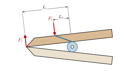
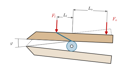
Example 4 took the turn of the legs as given. A designer starts from the forces instead. The peg of Figure 9.8.18 (a) should grip the cloth with a force \(F_c = 3\) N at the jaw tips, \(L_c = 40\) mm from the coil axis, and open its jaws by \(\varphi = 8^\circ\) under a finger force \(F_o = 11\) N at \(L_o = 25\) mm. A peg whose spring is free when the jaws touch would grip nothing, so the spring is already wound up by a preload angle\(\varphi_0\) when the peg is closed. We find the preload and the rate \(k\) that meet both requirements, and compare them with the spring of Example 4.
(a) A wooden clothes peg held open.
(b) Closed, with the jaws in contact.
(c) Held open by the angle \(\varphi\).
Figure 9.8.18: Example 5. The upper arm of a clothes peg turns about the coil axis. The leg of the spring presses on it with \(F_l\) at the arm \(L_l\), the lower jaw pushes back with \(F_c\) at \(L_c\), and the fingers press with \(F_o\) at \(L_o\).
The pin at the coil axis carries a force but no moment, so moment equilibrium of the upper arm about that axis involves only the spring leg and the applied force. With the peg closed, Figure 9.8.18 (b), the spring has turned by \(\varphi_0\) from its free position. Its leg presses with the moment \(F_l L_l = k\varphi_0\), and the jaws take it up,
\[
k\varphi_0 = F_c L_c = M_c
\tag{9.8.22}\]
Held open, Figure 9.8.18 (c), the spring has turned by a further \(\varphi\), and the fingers carry the larger moment,
The leg force and its arm have dropped out, since only their product, the moment of the spring, enters. Subtracting 9.8.22 from 9.8.23 eliminates \(\varphi_0\) and gives the rate, and 9.8.22 then gives the preload,
The moments cancel in \(\varphi_0\), so the preload is a fraction of the opening angle set by the ratio of the two moments alone. It is positive only when opening takes more moment than clamping provides, \(M_o > M_c\), and it grows without bound as the two moments approach each other.
Code
M_c, M_o, phi_0 = sp.symbols('M_c M_o varphi_0', positive=True)k = sp.symbols('k', positive=True) # the rate is now the unknownclosed = sp.Eq(k*phi_0, M_c) # @eq-peg-closed: wound up by phi_0, jaws shutopened = sp.Eq(k*(phi_0 + phi), M_o) # @eq-peg-open: turned a further phi by the fingerssol5 = sp.solve([closed, opened], [phi_0, k], dict=True)[0]
SymPy solves 9.8.22 and 9.8.23 for \(\varphi_0\) and \(k\), and the difference from 9.8.24 vanishes,
With \(M_c = 3 \cdot 40 = 120\) N mm, \(M_o = 11 \cdot 25 = 275\) N mm and \(\varphi = 8^\circ\),
Code
ex5 = {M_c: 3*40, M_o: 11*25, phi: 8*sp.pi/180} # N mm, N mm and rad
\[ \begin{aligned}\varphi_0 &=0.108~\text{rad} =6.19^\circ\\ k &=1110~\text{N\,mm/rad}\end{aligned} \]
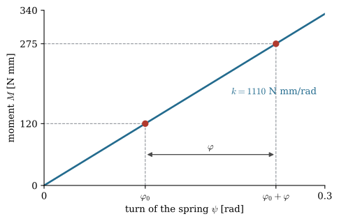
The two requirements are two points on the characteristic of the spring, Figure 9.8.19. The line through them must also pass through the origin, which is what fixes the preload: the slope between the points is \(k\) by 9.8.1, and the line through the origin with that slope reaches \(M_c\) at \(\varphi_0\).
Code
k_val =float(sol5[k].subs(ex5))p0 =float(sol5[phi_0].subs(ex5))p1 = p0 +float(ex5[phi])psi = np.linspace(0, 0.3, 50)fig, ax = plt.subplots(figsize=(5.4, 3.4))ax.plot(psi, k_val*psi, color=BLUE, lw=2)for p, M, txt in ((p0, 120, '$M_c$'), (p1, 275, '$M_o$')): ax.plot([p, p, 0], [0, M, M], color=GREY, lw=0.8, ls='--') ax.plot(p, M, 'o', color=RED)ax.annotate('', xy=(p1, 60), xytext=(p0, 60), arrowprops=dict(arrowstyle='<|-|>', color='0.3'))ax.text((p0 + p1)/2, 70, r'$\varphi$', ha='center')ax.text(0.2, k_val*0.2-45, f'$k = {k_val:.0f}$ N mm/rad', color=BLUE)ax.set_xlim(0, 0.3)ax.set_ylim(0, 340)ax.set_xticks([0, p0, p1, 0.3], ['0', r'$\varphi_0$', r'$\varphi_0 +\varphi$', '0.3'])ax.set_yticks([0, 120, 275, 340])ax.set_xlabel(r'turn of the spring $\psi$[rad]')ax.set_ylabel('moment $M$ [N mm]')for s in ('top', 'right'): ax.spines[s].set_visible(False)plt.show()
Figure 9.8.19: The characteristic \(M = k\psi\) of the peg spring. Closed, the spring is turned by \(\varphi_0\) and holds \(M_c\); open, it is turned by \(\varphi_0 + \varphi\) and holds \(M_o\).
A preload of about \(6^\circ\) and a rate of about \(1110\) N mm/rad meet both requirements. The spring of Example 4 has \(k = 1086\) N mm/rad, two percent less, and with the preload it turns through \(\varphi_0 + \varphi = 0.248\) rad when open, the \(0.25\) rad assumed there. That spring is the one this design calls for. The graph also shows what the preload does: it moves the working range of the spring up its characteristic, away from the origin where a closed peg would grip with no force at all.
Other spring types
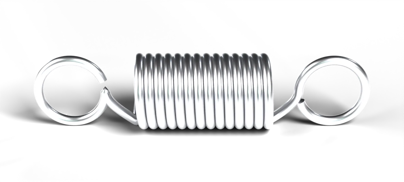
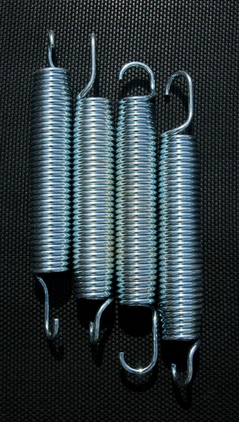
The extension spring is close wound, with a loop or a hook at each end, Figure 9.8.20. It is usually wound with an initial tension\(F_i\) that presses the coils together, so that it does not start to extend until the load exceeds \(F_i\), and its characteristic is \(F = F_i + k\delta\) with the rate of 9.8.9. The hooks, where the wire is bent sharply and loaded in bending as well as torsion, are where extension springs fail.
(a) An extension spring with machine loops.
(b) Trampoline springs.
Figure 9.8.20: Extension springs, close wound with a loop at each end.
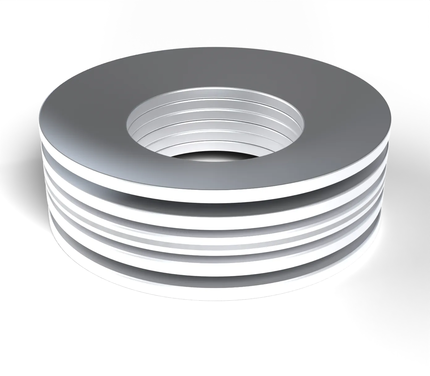
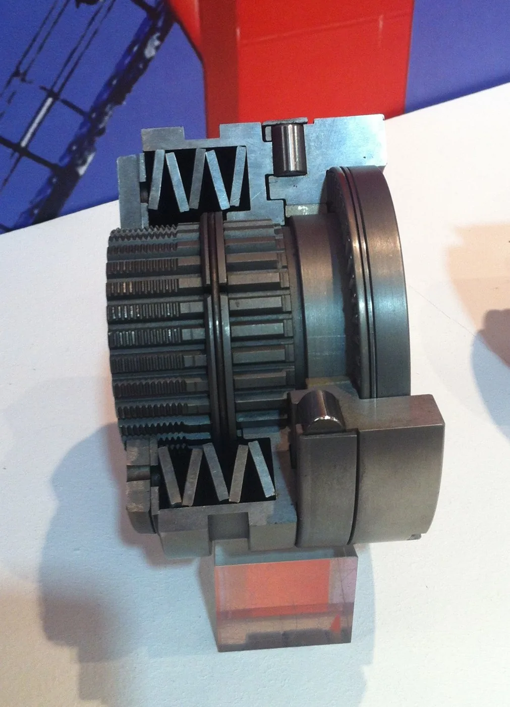
The disc spring, or Belleville washer, is a shallow coned annulus that flattens under an axial load, Figure 9.8.21. A single disc gives a large force over a small stroke, and the proportions of the cone decide whether its characteristic is nearly linear or markedly degressive1. Discs are stacked to tailor the result: discs facing alternately are in series and multiply the stroke, discs nested in the same direction are in parallel and multiply the force, and the rules for springs in series and in parallel apply directly. Disc stacks preload bolted joints and bearings, and set the slipping torque of torque limiters.
(a) Six disc springs stacked alternately, that is in series.
(b) A sectioned torque limiter with its disc spring stack.
Figure 9.8.21: Disc springs.
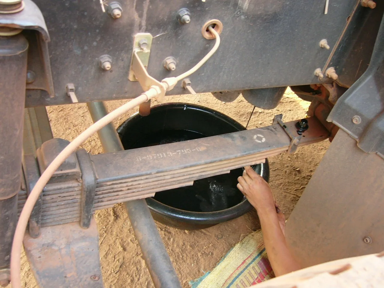
The leaf spring is a beam, and its rate follows from beam theory. A multi-leaf spring, Figure 9.8.22 (a), approximates a beam of constant bending stress: the leaves are stacked so that the depth of the stack follows the bending moment, which uses the material evenly along the length. Leaf springs also locate the axle they carry, and the friction between the leaves damps the motion.
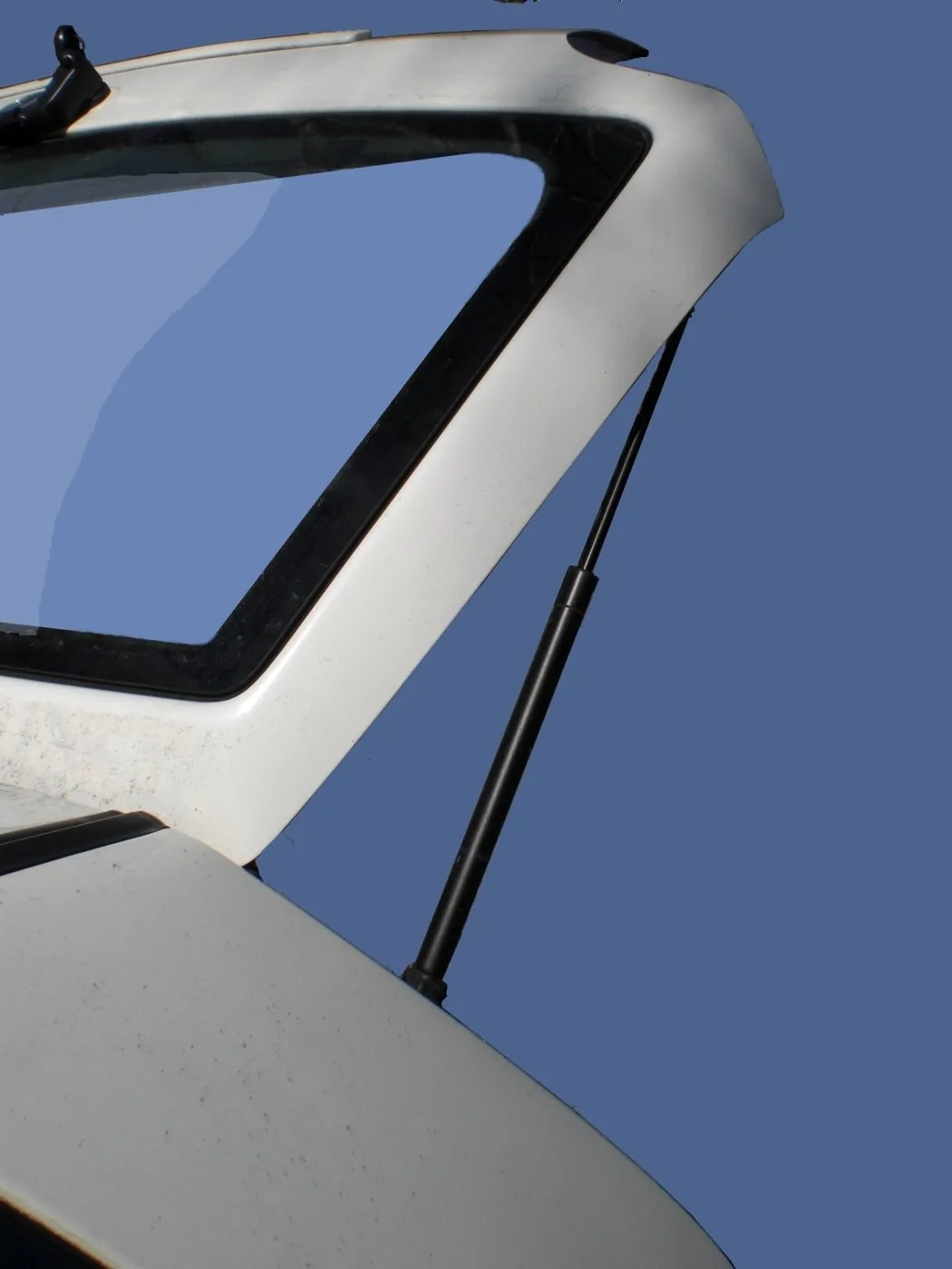
The gas spring, Figure 9.8.22 (b), is a cylinder of compressed nitrogen with a piston rod. The force is the gas pressure times the cross-section of the rod, \(F = pA\), and since the rod displaces only a small part of the gas volume, the pressure, and with it the force, rises only slightly over the stroke. Holding up a tailgate or a lid calls for that nearly constant force. An oil charge and a small orifice in the piston make it a damper as well.
The spiral spring of the clock in Figure 9.8.2 is a flat strip wound into a spiral and, like the torsion spring, loaded in bending, so its rate is \(EI/L\) for a strip of length \(L\).
(a) A multi-leaf spring on a truck.
(b) Gas springs on a hatchback tailgate.
Figure 9.8.22: Leaf and gas springs.
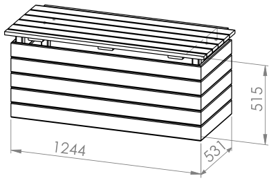
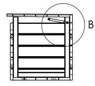
Example 6: Gas springs for a toy-box lid
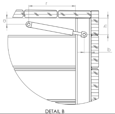
A toy box of pressure-treated timber, Figure 9.8.23, has a lid of mass \(m = 6.5\) kg and depth \(D = 524\) mm, hinged along its back edge. A child must be able to open and close it. Once lifted to about \(20^\circ\), the lid should open the rest of the way by itself, it must not slam shut, and it must not trap fingers. One gas spring on each side of the box carries the lid, Figure 9.8.23 (c). Each is pinned at \(B\), on a bracket that hangs \(a = 30\) mm below the point \(A\) of the lid, \(r = 205\) mm from the hinge, and at \(C\), on a bracket on the wall of the box, \(b = 30\) mm in front of and \(h = 55\) mm below the hinge. We choose the springs and adjust the mounting until the lid behaves as required.
(a) The toy box.
(b) Section through the box. The circle marks the corner shown in (c).
(c) The hinge corner, with the gas spring and its mounting.
Figure 9.8.23: Example 6. A toy box with a lid held up by two gas springs, dimensions in mm.
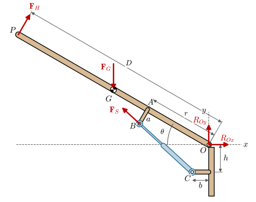
We place the origin at the hinge \(O\) and describe the lid opened by \(\theta\), Figure 9.8.24. The lid points along
and the bracket stands at right angles to it. Turning \(\bm e_{OA}\) by \(90^\circ\) anticlockwise with the rotation matrix gives the direction of the bracket,
Figure 9.8.24: Example 6. Free body of the lid, opened by \(\theta\). The two gas springs push along \(CB\) with the force \(\bm F_S\), and a hand lifts the front edge \(P\) with \(\bm F_H\) at right angles to the lid. Not to scale.
The two springs together push the lid with \(\bm F_S = F_S\,\bm e_{CB}\), and the weight is \(\bm F_G = -mg\,\bm e_y\). A hand at the front edge \(P\) lifts with \(\bm F_H = F_H\,\bm e_n\), where \(\bm e_n = d\bm e_{OA}/d\theta = [\sin\theta,\ \cos\theta]^\mathsf{T}\) is the direction in which the edge moves as the lid opens. The hinge reaction has no moment about \(O\), so moment equilibrium about the hinge gives one equation free of it,
The spring force acts at \(B\), but its moment may be taken through \(C\) instead, since both points lie on its line of action. The last term is \(-DF_H\,\bm e_z\), because lifting the lid turns it clockwise. 9.8.26 serves twice. With \(F_H = 0\) it gives the spring force \(F_{S,\text{req}}(\theta)\) that holds the lid still at \(\theta\) by itself, and once the springs are chosen it gives the hand force at every angle. The hinge reaction would follow from \(\sum\bm F = \bm 0\), but we do not need it.
Code
theta = sp.symbols('theta', real=True) # the opening angle of the lidb, h, r, m, g = sp.symbols('b h r m g', positive=True)F_S, F_H = sp.symbols('F_S F_H', real=True)e_OA = sp.Matrix([-sp.cos(theta), sp.sin(theta), 0])e_AB = sp.Matrix([[0, -1, 0], [1, 0, 0], [0, 0, 1]])*e_OA # e_OA turned 90 deg anticlockwisee_n = e_OA.diff(theta) # the way the front edge movesr_OB = r*e_OA + a*e_ABr_OC = sp.Matrix([-b, -h, 0])r_OG = D/2*e_OAr_OP = D*e_OAL_CB = (r_OB - r_OC).norm() # @eq-box-springe_CB = (r_OB - r_OC)/L_CBM_O = (r_OC.cross(F_S*e_CB) + r_OG.cross(sp.Matrix([0, -m*g, 0]))+ r_OP.cross(F_H*e_n))[2] # @eq-box-moment, z componentF_S_req = sp.solve(M_O.subs(F_H, 0), F_S)[0]F_H_th = sp.solve(M_O, F_H)[0]ex6 = {r: 205, D: 524, a: 30, b: 30, h: 55, m: 6.5, g: 9.81} # mm, kg and m/s^2
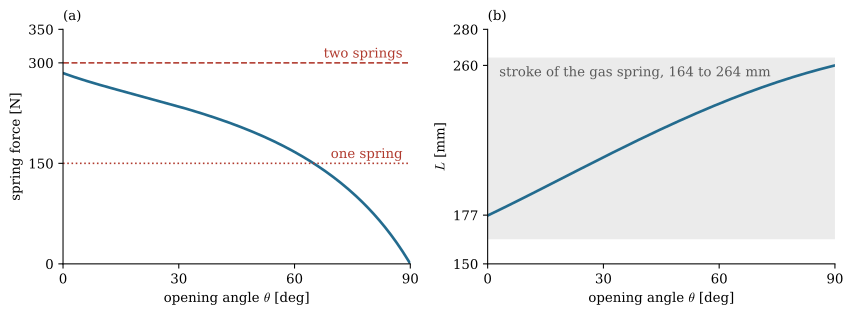
With the data of Figure 9.8.23 (c), the closed lid is held still by a spring force of
\[ F_{S,\text{req}}(0) =284.7~\text{N} \]
The required force falls as the lid opens, Figure 9.8.25 (a), because the arm of the weight about the hinge, \((D/2)\cos\theta\), shrinks faster than the arm of the spring. Over the whole opening the spring length of 9.8.25 runs from \(177\) to \(260\) mm, (b). A catalogue gas spring with an extended length of \(264\) mm and a stroke of \(100\) mm, and so a compressed length of \(164\) mm, covers that range, and it is stocked with the force \(F_1 = 150 \pm 20\) N2.
Code
deg = np.linspace(0, 90, 181)F_req_n = sp.lambdify(theta, F_S_req.subs(ex6))L_n = sp.lambdify(theta, L_CB.subs(ex6))fig, (ax1, ax2) = plt.subplots(1, 2, figsize=(9, 3.4))ax1.plot(deg, F_req_n(np.radians(deg)), color=BLUE, lw=2, label=r'$F_{S,\mathrm{req}}$')for F, ls, txt in ((300, '--', 'two springs'), (150, ':', 'one spring')): ax1.axhline(F, color=RED, ls=ls, lw=1.2) ax1.text(88, F +8, txt, ha='right', color=RED)ax1.set_ylim(0, 350)ax1.set_yticks([0, 150, 300, 350])ax1.set_ylabel('spring force [N]')ax2.plot(deg, L_n(np.radians(deg)), color=BLUE, lw=2)ax2.axhspan(164, 264, color='0.92', zorder=0)ax2.text(3, 254, 'stroke of the gas spring, 164 to 264 mm', color='0.35')ax2.set_ylim(150, 280)ax2.set_yticks([150, 177, 260, 280])ax2.set_ylabel('$L$ [mm]')for ax, t in ((ax1, '(a)'), (ax2, '(b)')): ax.set_xlim(0, 90) ax.set_xticks([0, 30, 60, 90]) ax.set_xlabel(r'opening angle $\theta$[deg]') ax.text(0, 1.04, t, transform=ax.transAxes)for s in ('top', 'right'): ax.spines[s].set_visible(False)plt.tight_layout()plt.show()
Figure 9.8.25: The spring force and the spring length against the opening angle. (a) The force that holds the lid still by itself, against the force of one and of two catalogue springs. (b) The length \(CB\) of the spring against the range of the catalogue spring.
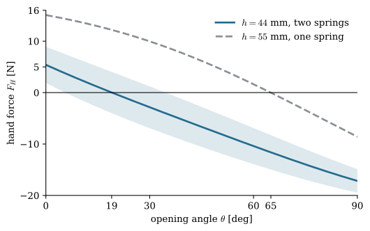
Two such springs give \(300\) N, more than the \(285\) N the closed lid needs, so the lid would lift off its seat unaided and could not be shut. A single spring gives \(150\) N and the lid stays shut, but the hand must carry it all the way to \(65^\circ\) before the spring takes over, Figure 9.8.26. The catalogue fixes the force, while the mounting is ours to choose. Raising the wall bracket from \(h = 55\) to \(44\) mm shortens the arm of the spring force about the hinge at small angles, so that two springs no longer lift the closed lid. At \(90^\circ\) the arm is \(b\) whatever \(h\) is, and the open lid is unaffected.
Code
F_H_one = F_H_th.subs(ex6).subs(F_S, 150) # original bracket, one springF_H_two = F_H_th.subs({**ex6, h: 44, F_S: 300}) # raised bracket, two springstheta_bal = sp.nsolve(F_H_two, theta, 0.3) # where the springs take over
For the raised bracket with two springs, the hand force at the closed and the fully open lid and the angle at which the springs take over are
rad = np.radians(deg)F_H_n = sp.lambdify((theta, F_S), F_H_th.subs({**ex6, h: 44}))F_H_one_n = sp.lambdify(theta, F_H_one)fig, ax = plt.subplots(figsize=(6, 3.6))ax.fill_between(deg, F_H_n(rad, 260), F_H_n(rad, 340), color=BLUE, alpha=0.15, lw=0)ax.plot(deg, F_H_n(rad, 300), color=BLUE, lw=2, label='$h = 44$ mm, two springs')ax.plot(deg, F_H_one_n(rad), color=GREY, lw=2, ls='--', label='$h = 55$ mm, one spring')ax.axhline(0, color='k', lw=0.8)ax.set_xlim(0, 90)ax.set_ylim(-20, 16)ax.set_xticks([0, 19, 30, 60, 65, 90])ax.set_yticks([-20, -10, 0, 5, 10, 16])ax.set_xlabel(r'opening angle $\theta$[deg]')ax.set_ylabel('hand force $F_H$ [N]')ax.legend(frameon=False)for s in ('top', 'right'): ax.spines[s].set_visible(False)plt.show()
Figure 9.8.26: The hand force at the front edge of the lid, positive when lifting. The shaded band covers the force tolerance of \(\pm 20\) N on each of the two springs.
The closed lid now needs a lift of about \(5\) N at its front edge, the springs take over at \(19^\circ\), and pulling the open lid down takes at most \(17\) N, all within a child’s strength. Below \(19^\circ\) the lid settles under a moment no larger than that of the \(5\) N edge force, and the oil in the gas springs limits its speed, so it does not slam. Above \(19^\circ\) the lid stays up, which keeps fingers out of the gap. The spring length now runs from \(176\) to \(249\) mm, inside the stroke.
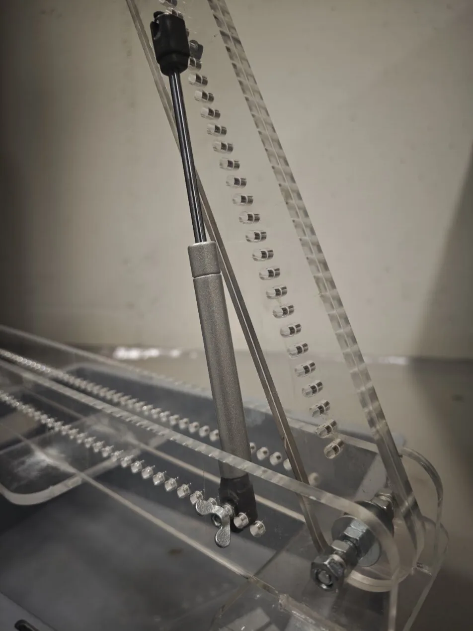
The band in Figure 9.8.26 is the catch. The tolerance of \(\pm 20\) N on each spring moves the angle at which the lid opens by itself anywhere between \(6^\circ\) and \(35^\circ\), so the tolerance matters more than the nominal force. Either a tighter tolerance is specified, or the springs are measured and the wall bracket gets a row of holes along \(h\) to set the balance on the assembled box, as on the demonstration rig of Figure 9.8.27. The catalogue force is also measured near full extension. A gas spring pushes somewhat harder as it is compressed, which lowers the balance angle further, and its data sheet gives the increase as the progression of the spring.
Figure 9.8.27: A demonstration rig for a gas-spring lid. Rows of holes in the lid and in the base let both ends of the gas spring be moved, which changes the arm of the spring force about the hinge.
Printed springs
Everything above holds for a printed spring, with two differences that matter. The first is the modulus. PLA has a shear modulus of roughly \(1.3\) GPa against \(79\) GPa for spring steel, so 9.8.9 makes a printed coil of the same geometry some sixty times softer, and a printed coil spring of useful stiffness needs a thick wire and few coils. The second is time. A polymer under constant strain relaxes, so a printed spring that holds a preload loses part of it within hours, and one held under constant load creeps. Printed springs suit loads that come and go, and should not be trusted to hold a preload over months.
A printed coil spring is also awkward to print, since each coil overhangs the one below. The form that suits the process is the flexure: a thin beam that bends, printed so that its bending stress runs along the layers, as in the compliant mechanism of Figure 9.8.28. Its rate is that of a cantilever, \(k = 3EI/L^3\), and the whole mechanism is one part with no joints to wear.
Figure 9.8.28: A printed compliant mechanism. The thin beams are flexures that act as springs and hinges at once.
Further reading
Shigley’s chapter on mechanical springs covers wire strengths, fatigue of springs and the design procedure in detail [1]. Wahl’s book is the classic treatment of the curvature correction and of the less common spring types [2]. The tables of spring dimensions and allowable stresses used in Swedish practice are collected by Björk [4].
Wahl AM. Mechanical springs. 2nd ed. New York: McGraw-Hill; 1963.
[3]
Haringx JA. On highly compressible helical springs and rubber rods, and their application for vibration-free mountings, I. Philips Research Reports 1948;3:401–49.
[4]
Björk K. Formler och tabeller för mekanisk konstruktion. 9th ed. Spånga: Karl Björks förlag HB; 2022.
The load-deflection relation of the disc spring is due to J. O. Almen and A. László, The uniform-section disk spring, Transactions of the ASME 58 (1936).↩︎