“On ne trouvera point de Figures dans cet Ouvrage. Les méthodes que j’y expose ne demandent ni constructions, ni raisonnemens géométriques ou méchaniques, mais seulement des opérations algébriques, assujetties à une marche réguliere & uniforme.”
“No figures will be found in this work. The methods I set out in it require neither constructions nor geometrical or mechanical reasoning, but only algebraic operations, subject to a regular and uniform procedure.”
The pendulum on the cart in Rigid body kinetics needed two free body diagrams, five equations and five unknowns, three of which were forces nobody had asked for. Virtual work showed why those forces can be left out: the ideal constraints do no virtual work. This chapter turns that observation into a method. The equations of motion of a system follow from two scalar functions, its kinetic and its potential energy, by a fixed recipe of differentiations, one equation for each degree of freedom and none for the reactions.
The recipe comes from a question that occupied mathematicians for a century, and the chapter starts there.
Of all possible paths, which one?
A system moves from one configuration \(A\) at the time \(t_1\) to another, \(B\), at the time \(t_2\). Of all the ways it could have gone between them, which one does it take? Newton’s answer works forward in time: from the forces now, find the acceleration now, and step on. The question above looks at the whole path at once, and its answer is a statement about the path as a whole.
NoteThe story of least action
In June 1696 Johann Bernoulli printed a challenge in the Acta Eruditorum, the journal of the learned world. A bead slides without friction from one point to a lower point that is not directly below it: along which curve does it arrive soonest? The straight line is the shortest path but not the quickest. A path that drops steeply at first lets the bead pick up speed early, and it wins although it is longer.
Isaac Newton, by then Warden of the Mint, received the problem in late January 1697. According to John Conduitt, the husband of Newton’s niece, he came home from the Mint at four in the afternoon, very tired, and did not go to bed until he had solved it, at four in the morning. His solution appeared without his name in the Philosophical Transactions, and Bernoulli is said to have recognised the author anyway, tanquam ex ungue leonem, as the lion by its claw.
The curve is a cycloid, the path of a point on the rim of a rolling wheel. Bernoulli’s own solution was the more surprising one. He treated the falling bead as a ray of light passing through layers of glass in which light moves faster the deeper it goes, and borrowed Pierre de Fermat’s principle of 1662: light travels between two points along the path of least time, and the law of refraction follows from that alone. The bead, like the light, takes the quickest path.
If light minimises time, what do bodies minimise? In 1744 Pierre-Louis Moreau de Maupertuis told the Paris Academy that nature economises a quantity he called action, mass times speed times distance, and two years later, as president of the Berlin Academy, he presented it as proof of a wise creator. It brought him ridicule. Samuel König claimed that Leibniz had known the principle first, the dispute became a scandal, and in 1752 Voltaire mocked Maupertuis in the Diatribe du docteur Akakia.
The mathematics had meanwhile been done without the theology. In 1744 Leonhard Euler showed that a body moving under central forces follows the path along which \(\int m v\,ds\) is stationary. In August 1755 a nineteen-year-old in Turin, Joseph-Louis Lagrange, wrote to Euler with a general method for such problems: vary the whole path by a small function and require the first-order change to vanish. Euler adopted it and named the subject the calculus of variations. Lagrange’s Méchanique analitique of 1788 built all of mechanics on it, without a single figure. In 1834 William Rowan Hamilton gave the principle the form this chapter uses, with the time integral of \(T - V\).
Least turned out to be the wrong word. The true path makes the action stationary: over short enough time intervals it is a minimum, but over longer ones it can be a saddle point, and the motion is the same. Richard Feynman heard about the principle from his high-school physics teacher, Mr. Bader, and it stayed with him. His 1948 formulation of quantum mechanics lets a particle take every path at once; the paths near the one of stationary action reinforce each other and the others cancel, which is why the path we see is the classical one. Veritasium tells the whole story in the video below.
The action and the Lagrangian
For a system with one generalised coordinate \(q(t)\), the kinetic energy \(T(q, \dot q)\) and the potential energy \(V(q)\) define the Lagrangian
The action is a number that depends on the whole function \(q(t)\), which the square brackets indicate. Hamilton’s principle states that of all paths with \(q(t_1) = q_A\) and \(q(t_2) = q_B\), the one the system takes makes the action stationary: a small change of the path changes \(S\) only to second order. We write the Lagrangian as \(\mathcal{L}\) to keep it apart from the lengths \(L\) of the examples.
Deriving the Euler-Lagrange equation
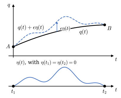
Let \(q(t)\) be the true path and compare it with a neighbouring path \(q(t) + \epsilon\,\eta(t)\), where \(\epsilon\) is a small number and \(\eta(t)\) any smooth function that vanishes at both ends, \(\eta(t_1) = \eta(t_2) = 0\), so the varied path starts and ends where the true one does (Figure 7.9.1).
Figure 7.9.1: The true path \(q(t)\) from \(A\) to \(B\), a varied path \(q + \epsilon\eta\) with the same end points, and the variation \(\eta(t)\), which vanishes at \(t_1\) and \(t_2\).
On the varied path the Lagrangian is \(\mathcal{L}(q + \epsilon\eta,\ \dot q + \epsilon\dot\eta)\). A Taylor expansion in \(\epsilon\) gives
For the action to be stationary, \(\delta S\) must vanish for every \(\eta\). If the bracket were different from zero at some instant, an \(\eta\) concentrated around that instant would make the integral non-zero, so the bracket must vanish everywhere:
This is the Euler-Lagrange equation. For a system with the coordinates \(q_1, \dots, q_n\), each is varied on its own and each gives one equation of the form 7.9.1.
The variation \(\epsilon\eta(t)\) is the virtual displacement \(\delta q\) of Virtual work: small, arbitrary, and zero where the motion is prescribed. The derivation also has the three steps that the finite element method uses to turn a differential equation into its weak form: multiply by an arbitrary function, integrate by parts, and drop the boundary term because the function vanishes where the solution is prescribed. In the finite element method the arbitrary function is a virtual displacement in space instead of in time, and the vanishing boundary term says that a support does no work.
Forces that are not conservative
A damper, friction, or a motor has no potential energy, and Hamilton’s principle in the form above cannot include it. Its virtual work can. For each coordinate, the virtual work of the non-conservative forces defines a generalised force \(Q\) as in Virtual work, \(\delta U_{\text{nc}} = Q\,\delta q\). Adding this work to the variation of the action, \(\int_{t_1}^{t_2}(\delta\mathcal{L} + Q\,\delta q)\,dt = 0\), and repeating the steps above puts \(Q\) on the right-hand side:
A viscous damper with the coefficient \(c\) acting on the rate \(\dot q\) gives \(Q = -c\dot q\); an applied force or moment gives its virtual work per unit \(\delta q\).
The recipe
The method is the same for every system:
Choose the generalised coordinates \(q_1, \dots, q_n\), one per degree of freedom.
Write the kinetic energy \(T\) and the potential energy \(V\) in the coordinates and their rates.
Form \(\mathcal{L} = T - V\) and find the generalised forces \(Q_j\) of the non-conservative forces from their virtual work.
Differentiate: \(\dfrac{d}{dt}\dfrac{\partial\mathcal{L}}{\partial\dot q_j} - \dfrac{\partial\mathcal{L}}{\partial q_j} = Q_j\) for each \(j\).
The first three steps are modelling and need the mechanics. The fourth is mechanical differentiation, which SymPy does.
Example 1: The collar
The collar of Example 1 in Work, energy and power (Figure 7.3.1) has one degree of freedom, the angle \(\theta\), and no friction. Its speed is \(r\dot\theta\), its height above \(2\) is \(r(1 - \sin\theta)\), and its spring has the length \(\ell(\theta) = \sqrt{d^2 + 2dr\cos\theta + r^2}\):
\[
T = \tfrac{1}{2}m r^2\dot\theta^2 , \qquad
V = mgr\,(1 - \sin\theta) + \tfrac{1}{2}k\bigl(\ell(\theta) - d\bigr)^2 .
\]
7.9.1 with \(\mathcal{L} = T - V\) gives the equation of motion, which we compare with the one Newton’s second law gave in 7.3.1.
Code
t = sp.symbols('t', real=True)m, r, d, k, g = sp.symbols('m r d k g', positive=True)def euler_lagrange(Lag, qs, Qs):"""The Euler-Lagrange equations d/dt(dL/dq') - dL/dq = Q, one per coordinate."""return [sp.Eq(sp.diff(Lag.diff(q.diff(t)), t) - Lag.diff(q), Q) for q, Q inzip(qs, Qs)]th = sp.Function('theta')(t)ell = sp.sqrt(d**2+2*d*r*sp.cos(th) + r**2)T1 = m*r**2*th.diff(t)**2/2V1 = m*g*r*(1- sp.sin(th)) + k*(ell - d)**2/2eq1, = euler_lagrange(T1 - V1, [th], [0])thdd_el = sp.solve(eq1, th.diff(t, 2))[0]thdd_newton = g/r*sp.cos(th) + k*d/(m*r)*(1- d/ell)*sp.sin(th) # eq-we-collarnamed = {th.diff(t, 2): sp.Symbol(r'\ddot\theta'), th.diff(t): sp.Symbol(r'\dot\theta'), th: sp.Symbol(r'\theta')}
The Euler-Lagrange equation and its difference from Newton’s result are
\[ \begin{aligned}\ddot\theta &=\dfrac{- \dfrac{d^{2} k \sin{\left(\theta \right)}}{\sqrt{d^{2} + 2 d r \cos{\left(\theta \right)} + r^{2}}} + d k \sin{\left(\theta \right)} + g m \cos{\left(\theta \right)}}{m r}\\ \ddot\theta_{\text{Lagrange}} - \ddot\theta_{\text{Newton}} &=0\end{aligned} \]
Two energies and one differentiation give the equation that took a free body diagram, two unit vectors and a projection in Example 1 of Work, energy and power. The normal force of the guide never appears, because it does no work.
Example 2: The bar pendulum, both ways
The bar pendulum of Example 1 in Rigid body kinetics (Figure 7.6.2) turns about the fixed pin \(O\) with the angle \(\theta\) from the downward vertical, and the pin resists with the friction moment \(-c\dot\theta\). Newton-Euler took moments about \(O\) to avoid the pin force:
With Lagrange, the kinetic energy of a body turning about a fixed pin is \(T = \tfrac12 I_O\dot\theta^2\), the potential energy of the weight is \(V = -mg\,r_G\cos\theta\) with the zero level at \(O\), and the friction moment does the virtual work \(-c\dot\theta\,\delta\theta\), so \(Q = -c\dot\theta\).
\[ \begin{aligned}I_{O} \ddot\theta + \dot\theta c + g m r_{G} \sin{\left(\theta \right)} = 0\end{aligned} \]
the Newton-Euler equation, with every term moved to the left. For one rigid body on a fixed pin the two methods are equally short, and the choice is a matter of taste. Newton-Euler gives the pin force on the way if the other two equations are written down, which Lagrange does not. Lagrange becomes the shorter route when bodies are connected, because every ideal connection removes its reactions from the work.
Example 3: The spring-damper system
The mass \(m\) on a spring \(k\) with a damper \(c\) in Example 6 in Particle kinetics (Figure 7.2.9) has one coordinate, the position \(x\) of the mass. With an external force \(F\) on the mass,
\[
T = \tfrac{1}{2}m\dot x^2 , \qquad V = \tfrac{1}{2}kx^2 , \qquad Q = -c\dot x + F ,
\]
since the damper and the external force do the virtual work \((-c\dot x + F)\,\delta x\).
\[ \begin{aligned}- F + \ddot x m + \dot x c + k x = 0\end{aligned} \]
the equation of motion of Particle kinetics, with the damper as a generalised force and the spring in the potential energy. The spring could have gone into \(Q\) as well, as \(-kx\); it is conservative, so its potential energy is the shorter route.
Example 4: The pendulum on the cart, and a tuned mass damper
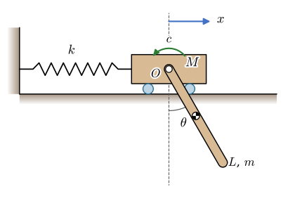
The pendulum on the sliding cart of Example 2 in Rigid body kinetics has the coordinates \(x\) and \(\theta\), with \(M = 10\) kg, \(k = 270\) N/m, a bar of \(m = 1\) kg and \(L = 0.6\) m. Here we add a rotational damper \(c\) in the pin (Figure 7.9.2), which resists the rotation of the bar relative to the cart. The cart does not rotate, so the relative rotation rate is \(\dot\theta\) and the damper does the virtual work \(-c\dot\theta\,\delta\theta\).
Figure 7.9.2: The pendulum on the cart with a rotational damper \(c\) in the pin \(O\).
Step 1 - Energies and the equations of motion
The cart moves with \(\dot x\). The centre of mass of the bar is at \(\bm r_G = [x + \tfrac{L}{2}\sin\theta,\ -\tfrac{L}{2}\cos\theta]^\mathsf{T}\), it turns with \(\dot\theta\), and \(\bar I = mL^2/12\). With 7.6.5 for the bar,
Two equations, written from two energies, where Newton-Euler needed five with three reactions. The first equation is the cart’s: its inertia \((M + m)\ddot x\), the coupling to the swing of the bar, and the spring. The second is the bar’s, and \(c\dot\theta\) appears in it alone, the generalised force of the damper.
Step 2 - The pendulum as a tuned mass damper
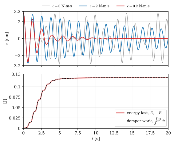
In Rigid body kinetics the cart and the bar traded their energy back and forth without loss. The damper in the pin turns that exchange into a way to remove vibration from the cart. We hold the bar vertical, push the cart to \(x_0 = 3\) cm and release both, and integrate with Euler-Cromer as before, for three damper coefficients. The energy check now has to account for the damper, which takes the work \(\int c\,\dot\theta^2\,dt\) out of the system:
\[
E_0 - E(t) = \int_0^t c\,\dot\theta^2\,dt , \qquad
E = T + V .
\]
amp = {cv: np.max(np.abs(runs[cv][1][(runs[cv][0] >18)])) for cv in runs}mismatch = np.max(np.abs((runs[0.2][3][0] - runs[0.2][3]) - runs[0.2][4]))
Without the damper (grey) the cart’s vibration drains into the bar and comes back, and after 20 s the cart still swings with its full amplitude. With \(c = 0.2\) N·m·s (red) the energy that reaches the bar is dissipated in the pin, and the cart has practically stopped after ten seconds. A stiffer damper is worse, not better: with \(c = 2\) N·m·s (blue) the damper nearly locks the bar to the cart, little relative rotation is left to dissipate, and the cart keeps swinging. The cart amplitudes over the last two seconds, and the largest mismatch of the energy check, are
\[ \begin{aligned}\max|x|\big|_{t>18\,\text{s}} &:\quad c = 0:\ 2.98~\text{cm},\quad c = 0.2:\ 0.01~\text{cm},\quad c = 2:\ 1.19~\text{cm}\\ \max\Bigl|(E_0 - E) - \int c\dot\theta^2\,dt\Bigr| &\approx3.0 \cdot 10^{-5}~\text{J}\end{aligned} \]
This is a tuned mass damper: a small mass on a spring or a pendulum, tuned to the frequency of the structure, with a damper chosen to dissipate as much as possible. Buildings, bridges and wind turbine towers carry them, and the best damper lies between too weak and too stiff, as the three curves show.
Energy from the Lagrangian
The energy balance of Work, energy and power was derived from Newton’s second law. It also follows from the Euler-Lagrange equations. Define the energy function
When the Lagrangian does not depend on time explicitly, \(h\) changes only through the power \(\sum_j Q_j\dot q_j\) of the non-conservative forces, and without them it is constant. In our examples \(T\) is a quadratic form in the rates \(\dot q_j\), for which \(\sum_j\dot q_j\,\partial T/\partial\dot q_j = 2T\), and \(V\) does not depend on the rates, so
\[
h = 2T - (T - V) = T + V .
\]
The conserved quantity is the total mechanical energy, and for the cart with its damper \(dh/dt = -c\dot\theta^2\), the rate at which the damper dissipates, which the energy check above confirmed. Expressed in the coordinates and their momenta \(\partial\mathcal{L}/\partial\dot q_j\), \(h\) is the Hamiltonian, the function at the centre of Hamilton’s reformulation of mechanics. For the cart we check \(h = T + V\) directly:
Code
h4 =sum(q.diff(t)*(T4 - V4).diff(q.diff(t)) for q in (x4, th4)) - (T4 - V4)h_check = sp.simplify(h4 - (T4 + V4))
\[ \begin{aligned}h - (T + V) &=0\end{aligned} \]
Small oscillations
Near a stable equilibrium the motion is small and the equations can be linearised. For coordinates measured from the equilibrium, the kinetic energy at small rates and the potential energy near its minimum are quadratic forms,
and the Euler-Lagrange equations become \(\bm M\ddot{\bm q} + \bm K\bm q = \bm 0\). Trying \(\bm q = \hat{\bm q}\cos\omega t\) gives the eigenvalue problem \((\bm K - \omega^2\bm M)\hat{\bm q} = \bm 0\), whose roots are the natural frequencies of the system. The mass matrix\(\bm M\) and the stiffness matrix\(\bm K\) are the matrices of the same names in the finite element method, and the eigenvalue problem is its modal analysis.
For the cart without damper the two frequencies explain the energy exchange of Rigid body kinetics. The spring was tuned so that the cart and the bar alone have the same frequency; coupled, they split into two frequencies close to each other, and the exchange repeats with their beat period \(2\pi/(\omega_2 - \omega_1)\).
The mass and stiffness matrices, and with the numbers of the example the frequencies and the beat period, are
\[ \begin{aligned}\bm M &=\left[\begin{matrix}M + m & \dfrac{L m}{2}\\\dfrac{L m}{2} & \dfrac{L^{2} m}{3}\end{matrix}\right],\quad \bm K =\left[\begin{matrix}k & 0\\0 & \dfrac{L g m}{2}\end{matrix}\right]\\ \omega_1 &=4.41~\text{rad/s},\quad \omega_2 =5.76~\text{rad/s},\quad \frac{2\pi}{\omega_2 - \omega_1} =4.65~\text{s}\end{aligned} \]
The beat period of 4.65 s is the time in which the bar of Rigid body kinetics handed its swing to the cart and took it back.
TipIn industry: the manipulator equation
Model-based robot control uses the Euler-Lagrange equation of the arm in matrix form, \(\bm M(\bm q)\ddot{\bm q} + \bm C(\bm q, \dot{\bm q})\dot{\bm q} + \bm g(\bm q) = \bm\tau\), with the mass matrix \(\bm M\) from the kinetic energy, the velocity terms \(\bm C\), the gravity terms \(\bm g\) from the potential energy and the joint moments \(\bm\tau\) as generalised forces. General-purpose programs such as SolidWorks Motion and Adams typically take another route, described in How a motion solver works.
From here
How a motion solver works keeps every body free and the reactions in the equations, which suits a program that must handle any mechanism. Energy methods applies virtual work to bodies that deform, and the finite element method takes the three steps of the derivation above into space.
Further reading
Feynman’s lecture on the principle of least action, chapter 19 of volume II of The Feynman Lectures on Physics, is free at https://www.feynmanlectures.caltech.edu/II_19.html and tells the story of how he learned it. Goldstein, Poole and Safko [1] derive the Euler-Lagrange equations from d’Alembert’s principle and from Hamilton’s principle, and treat small oscillations and the Hamiltonian in full.
References
[1]
Goldstein H, Poole CP, Safko JL. Classical mechanics. 3rd ed. San Francisco: Addison Wesley; 2002.