An electric motor runs fast with little torque, and a wheel, a winch drum or a conveyor needs the opposite. A transmissionsv. transmission sits between them and trades one for the other: the motor is the source of the power, the machine the consumer, and the transmission changes speed and torque on the way while passing the power on, less what it loses in friction. Belts and chains do this between shafts far apart, as the chapter on belt drives shows. Gears do it between shafts close together, with teeth that cannot slip.
This chapter starts from the relation between power, torque and speed, and the speed ratio of a pair of gears, using the gear train of Figure 9.4.1. It then takes the other kinds of gear pairs in turn: the worm drive, for large ratios between crossed shafts, the bevel gear pair, for shafts that meet, and the differential built from bevel gears, which lets the wheels of a car turn at different speeds. The last part is the strength of the teeth: the forces on a tooth, Lewis’s classical estimate of the bending stress at its root, a finite element model of two gears in mesh that shows how the load moves over the teeth as they turn, and the load diagram of a gear catalogue built from the root and flank limits.
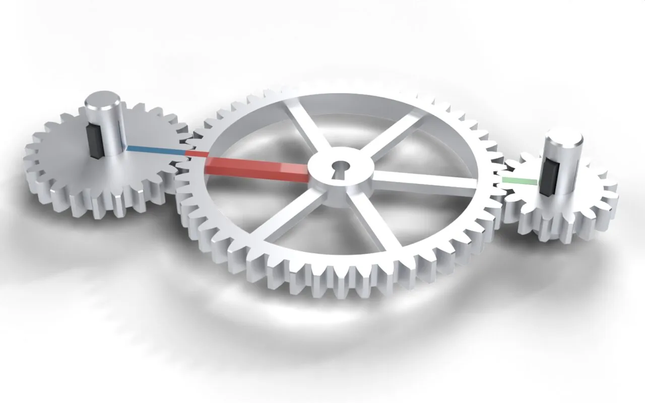
Figure 9.4.1: A train of three spur gears with 24, 48 and 16 teeth. The pitch radii are painted on: blue on the left gear, the red spoke of the middle gear, green on the right gear. They start in line and turn apart, each gear at its own speed. The black keys on the shafts show that the outer gears turn their shafts; the middle gear turns freely on a pin through its keyhole.
Power, torque and speed
A torque \(T\) on a shaft turning at the angular velocity \(\omega\) delivers the power
\[
P = T\,\omega
\tag{9.4.1}\]
with \(\omega\) in rad/s. Speeds are usually given in revolutions per minute, \(n\), and \(\omega = 2\pi n/60\). A transmission that changes the speed by the ratiosv. utväxling\(i = \omega_\text{in}/\omega_\text{out}\) and loses nothing must deliver the same power at its output, \(T_\text{out}\,\omega_\text{out} = T_\text{in}\,\omega_\text{in}\), so the torque changes by the same ratio the other way. A real transmission loses a part of the power, which the efficiencysv. verkningsgrad\(\eta\) accounts for:
\[
i = \frac{\omega_\text{in}}{\omega_\text{out}}, \qquad
T_\text{out} = \eta\, i \, T_\text{in}
\tag{9.4.2}\]
A pair of good spur gears has \(\eta \approx 0.98\) to \(0.99\); the losses are the sliding of the flanks against each other and the churning of the oil.
For a pair of gears, the ratio follows from the pitch circles of the chapter on spur gears. The two pitch circlessv. delningscirklar touch at the pitch point on the line between the centres and roll on each other without slipping, so a point on each moves with the same speed there, \(\omega_1 r_1 = \omega_2 r_2\). With the pitch diameter \(d = mN\) for the module \(m\) and the number of teeth \(N\), which two meshing gears share,
\[
i = \frac{\omega_1}{\omega_2} = \frac{r_2}{r_1} = \frac{N_2}{N_1}
\tag{9.4.3}\]
The gears turn in opposite directions. The painted lines of Figure 9.4.1 are the pitch radii: at the start they lie along the line of centres and meet at the pitch points, and as the gears turn, the arcs they sweep on the pitch circles stay equal. In a train of several gears the ratios multiply, \(i = i_{12}\, i_{23} \cdots\), and the middle gear of Figure 9.4.1 shows what that implies for a gear that meshes with two others.
Example 1: the gear train
A motor of \(P = 1.5\) kW at \(n_1 = 1450\) rpm drives the left gear of Figure 9.4.1, \(N_1 = 24\), which drives the middle gear, \(N_2 = 48\), which drives the right gear, \(N_3 = 16\); the module is \(m = 3\) mm and the pressure angle \(20°\). Find the speed of each gear and the torque on the output shaft, first without losses and then with \(\eta = 0.98\) for each mesh. What force does a tooth carry, and what load does the middle gear put on its pin?
The speeds follow from 9.4.3, mesh by mesh, and the torques from 9.4.1 and 9.4.2. The force between the teeth acts along the line of action, at the pressure angle to the tangent of the pitch circles; its tangential part \(F_t = 2T/d\) carries the torque, and the radial part \(F_r = F_t\tan 20°\) pushes the gears apart.
Code
P_1, n_1 =1500, 1450# motor power [W] and speed [rpm]N_1, N_2, N_3, m =24, 48, 16, 3e-3# teeth, module [m]eta =0.98# efficiency per meshn_2 = n_1*N_1/N_2 # each mesh: n_in N_in = n_out N_outn_3 = n_2*N_2/N_3T_1 = P_1/(2*np.pi*n_1/60)T_3 = T_1*n_1/n_3 # same power, lower torque at the higher speedT_3_eta = eta**2*T_3 # two meshes on the wayF_t =2*T_1/(m*N_1) # tangential tooth force, the same in both meshesF_r = F_t*np.tan(np.radians(20))
The middle gear runs at half and the output at one and a half times the motor speed, and the torques are
The ratio from the motor to the output is \(n_1/n_3 = N_3/N_1 = 2/3\): the 48 teeth of the middle gear cancel out of the product \((N_2/N_1)(N_3/N_2)\). A gear that only passes motion on is an idlersv. mellanhjul. It changes the direction of the output and the distance between the shafts, never the ratio. It carries no torque either: the middle gear of Figure 9.4.1 turns freely on its pin, so the tooth forces on its two sides must have equal moments about it. At the left mesh the left gear pushes it with \(F_t\) on one side of the pin, and at the right mesh the output gear holds it back with \(F_t\) on the other side, so the two tangential forces point the same way and add up. The radial parts point at the pin from opposite sides and cancel. The pin of the idler carries \(2F_t \approx 550\) N, twice the tooth force, although the idler transmits no torque at all.
Kinds of gear pairs
Spur gearssv. rakkugghjul connect parallel shafts with straight teeth. A tooth comes into contact along its whole width at once and leaves the same way, and every change in the number of teeth in contact is a small knock; at high speed spur gears whine. Helical gearssv. snedkugghjul twist the teeth along the face, so a tooth enters gradually and more teeth share the load (9.4.19), at the price of an axial force on the bearings. The herringbone gear puts two helical halves of opposite hand side by side and cancels that force. Shafts that are not parallel need other kinds: the worm drive for shafts that cross, and the bevel gear for shafts that meet.
The worm drive
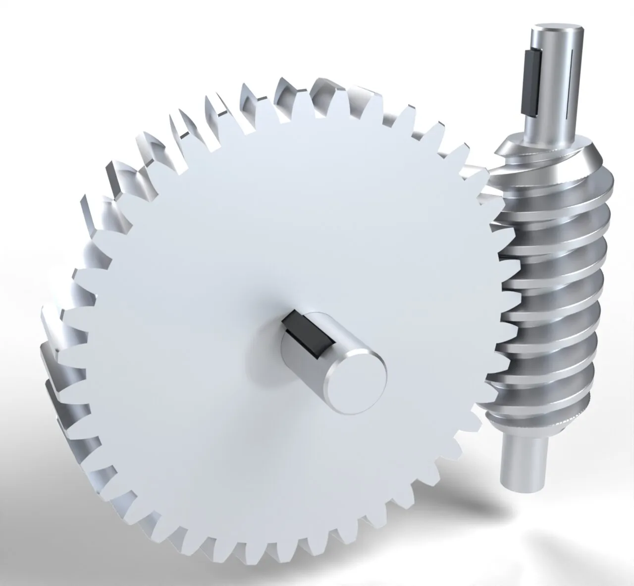
A wormsv. snäcka is a screw, and the worm wheelsv. snäckhjul it drives is a helical gear whose teeth fit its thread (Figure 9.4.2). One turn of a worm with \(z_1\) threads (or starts) moves the thread along by the lead \(z_1 p\), where \(p = \pi m\) is the axial pitch, and that turns the wheel by \(z_1\) teeth. The ratio is therefore
\[
i = \frac{N_2}{z_1}
\tag{9.4.4}\]
and a single pair makes ratios of 10 to 100 in a small box. The worm’s pitch diameter is not tied to its number of threads: it is \(d_1 = q\,m\) for a chosen diameter quotient\(q\), commonly 8 to 12. The thread climbs at the lead anglesv. stigningsvinkel\(\lambda\), the angle between the thread and the plane normal to the axis, which unrolling one turn of the pitch cylinder gives as
and the wheel’s teeth slope at the same angle, so the two mesh.
Figure 9.4.2: A two-start worm and its 40-tooth wheel, the drive of Example 2. The worm turns twenty times while the wheel turns once; the black key on the wheel shaft shows how slowly.
The thread does not roll on the wheel’s teeth, it slides along them, as a screw slides in its nut, and that makes the worm drive the least efficient of the gear pairs. Following [1], a force analysis of the thread as an inclined plane, with friction coefficient \(f\) and the normal pressure angle \(\varphi_n\) of the thread, gives the efficiency with the worm driving
which falls as the lead angle gets smaller. With the wheel driving, the roles of \(\tan\) and \(\cot\) swap, and the efficiency \((\cos\varphi_n - f\cot\lambda)/(\cos\varphi_n + f\tan\lambda)\) drops to zero when \(\tan\lambda \le f/\cos\varphi_n\). Then no torque on the wheel can turn the worm: the drive is self-lockingsv. självhämmande, and a hoist holds its load with the motor off.
Example 2: the worm drive
The worm of Figure 9.4.2 has \(z_1 = 2\) threads, axial module \(m = 4\) mm, \(q = 10\), a pressure angle of \(20°\) in the axial section, and drives a wheel with \(N_2 = 40\) teeth. Find the ratio, the lead angle, the centre distance and the efficiency for \(f = 0.05\), a steel worm on a bronze wheel in oil. Is the drive self-locking, and would a single-start worm be?
The normal pressure angle follows from the axial one through the lead angle, \(\tan\varphi_n = \tan\varphi\cos\lambda\).
Code
z_1, N_w, m_w, q, f =2, 40, 4.0, 10, 0.05def worm_drive(z_1): lam = np.arctan(z_1/q) # lead angle phi_n = np.arctan(np.tan(np.radians(20))*np.cos(lam)) eta = (np.cos(phi_n) - f*np.tan(lam))/(np.cos(phi_n) + f/np.tan(lam)) eta_back = (np.cos(phi_n) - f/np.tan(lam))/(np.cos(phi_n) + f*np.tan(lam))return np.degrees(lam), eta, eta_backi_w = N_w/z_1a_w = m_w*(q + N_w)/2# centre distance [mm], (d_1 + d_2)/2lam_2, eta_2, back_2 = worm_drive(2)lam_1, eta_1, back_1 = worm_drive(1)
For the two-start worm and, for comparison, a single-start worm, the results are
The two-start worm passes on 78 % of the power, and it can be driven backwards: neither drive is self-locking. Halving the number of starts halves the speed of the wheel and costs 13 percentage points of efficiency, yet the wheel can still drive the worm. Self-locking needs \(\tan\lambda \le f/\cos\varphi_n\), a lead angle below about \(3°\) with \(f = 0.05\), which means a single start and a large \(q\); and since \(f\) drops when the drive vibrates, a hoist does not rely on it but has a brake. A self-locking worm also has an efficiency below one half, so it turns more than half of the motor’s power into heat.
The bevel gear pair
Bevel gearssv. koniska kugghjul connect shafts whose axes meet, usually at a right angle, as in the differential of a car. The pitch circles of spur gears become pitch cones with a common apex where the axes meet, and the cones roll on each other along a common line (Figure 9.4.3). The speed ratio is again \(N_2/N_1\), and a cone’s pitch diameter at its back is still \(mN\), so the cone angles \(\delta_1 + \delta_2 = 90°\) must satisfy \(\tan\delta_1 = r_1/r_2 = N_1/N_2\):
The teeth taper towards the apex. Their shape at the back is approximately that of a spur gear on the back cone, the cone through the back end of the teeth perpendicular to the pitch cone, whose radius is \(r/\cos\delta\). Rolled out flat, the back cone is a spur gear with the virtual number of teeth
\[
N_v = \frac{N}{\cos\delta}
\tag{9.4.8}\]
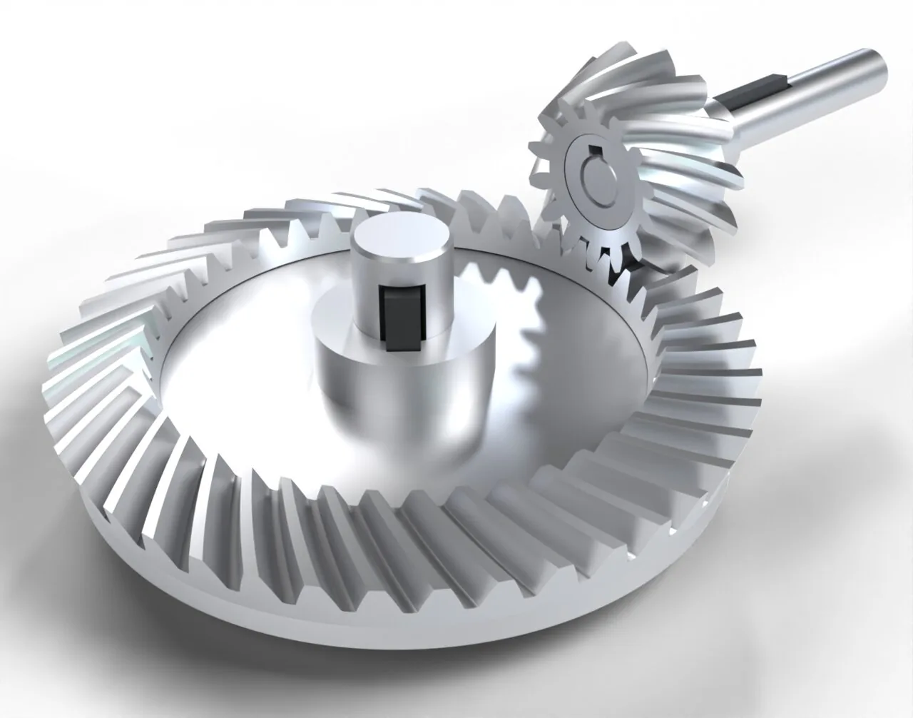
This is Tredgold’s approximation, and it is how bevel gears are designed with spur gear results, the tooth form, the undercut limit and the strength, and how the gears of Figure 9.4.3 were modelled. Straight teeth run along the cone towards the apex; the spiral bevel gears in the figure curve them, as helical teeth twist those of a spur gear, so they mesh more smoothly and quietly.
Figure 9.4.3: A spiral bevel gear pair of 14 and 42 teeth, the pair of Example 3, on keyed shafts that meet at a right angle. The spirals of the two gears have opposite hands.
Example 3: the bevel gear pair
The pinion of Figure 9.4.3 has \(N_1 = 14\) teeth and the wheel \(N_2 = 42\), module \(m = 4\) mm at the back and a face width of 24 mm. Find the cone angles, the cone distance from the apex to the back of the teeth, and the virtual numbers of teeth. Will the pinion’s teeth be undercut?
The face width of 24 mm is less than a third of the cone distance, the usual upper limit: a wider face would reach so far towards the apex that its inner end carries little load. The pinion acts like a spur gear of 14.8 teeth, below the 17 teeth that a \(20°\) involute needs to avoid undercut, so its teeth would be cut away at the root. Real bevel pinions avoid this with a profile shift, a longer addendum on the pinion and a shorter one on the wheel, which the model in the figure leaves out.
The differential
When a car turns, its outer wheels run on a larger circle than its inner wheels and must turn faster. On a corner of radius \(R\), measured to the middle of the axle, wheels a track width \(B\) apart run on the radii \(R \pm B/2\), and their speeds are in the ratio
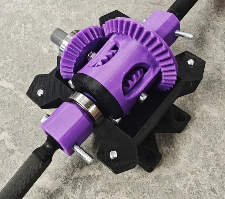
A solid axle forces both wheels to the same speed, so on every corner one of them slips, which wears the tyres and pushes the car straight on. The differentialsv. differential drives the two wheels through gears that let their speeds differ and still share the torque equally. The RC cars of the course project have one on each axle, made of printed bevel gears (Figure 9.4.4).
Figure 9.4.4: A differential printed in PLA, with its ring gear, the carrier with windows that show the spider gears, the bearings of the carrier and the half-shafts.
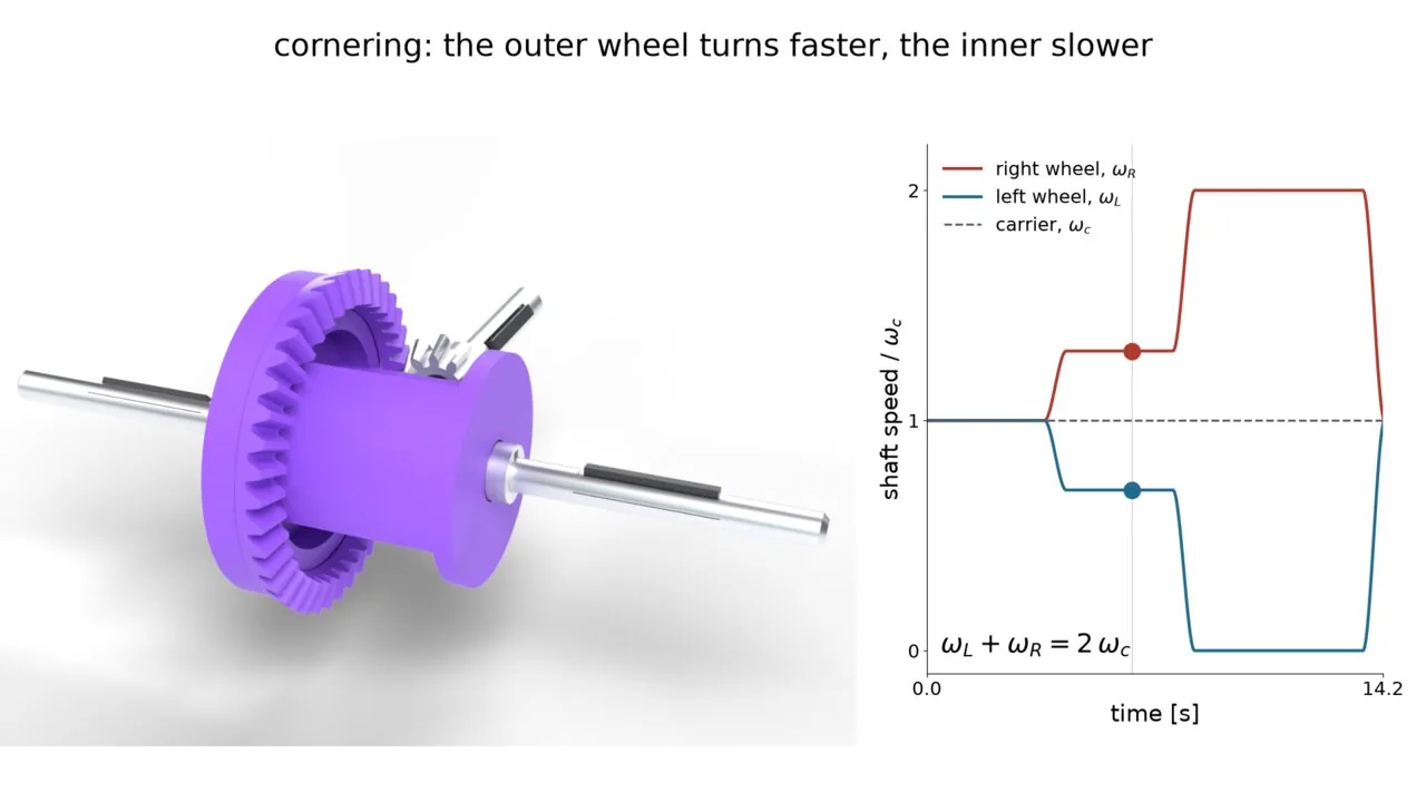
Figure 9.4.5 shows the open bevel-gear differential. The drive pinion turns the ring gear, a bevel wheel bolted to the carrier (purple), the housing that turns about the axle. The carrier holds a cross pin, and on it two spider gears turn freely. The spiders mesh with two side gears, one on each half-shaft. If the car drives straight, the spiders do not turn on their pin: they are wedges that carry the side gears round with the carrier, and everything turns as one block. If one wheel is slowed, its side gear lags the carrier, the spiders roll on it and drive the other side gear ahead by the same amount.
Figure 9.4.5: An open bevel-gear differential, driving straight ahead, through a corner, and with one wheel stuck. The ring gear (40 teeth) and the carrier turn at a constant speed; the spider gears (10 teeth) drive the side gears (16 teeth), whose half-shafts carry black keys. The graph shows the speeds of the two half-shafts and of the carrier.
The speeds follow from looking at the gears from the carrier, as if we rode on it. There the cross pin stands still, and the side gears and spiders form an ordinary train of bevel gears: side gear, spider, side gear. The two meshes multiply to the ratio \((N_\text{spider}/N_\text{side})(N_\text{side}/N_\text{spider}) = 1\), and the spider reverses the direction, so the two side gears turn equally fast in opposite directions relative to the carrier. Their speeds relative to the carrier are \(\omega_L - \omega_c\) and \(\omega_R - \omega_c\), so \(\omega_L - \omega_c = -(\omega_R - \omega_c)\), or
The carrier turns at the mean speed of the two wheels, and the wheels may share it out in any way. Each spider then turns on its pin at \((\omega_R - \omega_c)N_\text{side}/N_\text{spider}\).
The torques follow from the spider. It turns freely on its pin, so the two tooth forces on it, from the left and from the right side gear, must have equal moments about the pin: they are equal, and they act at the same radius on the two side gears. Neglecting friction, the torque of the carrier is therefore split equally,
\[
T_L = T_R = \frac{T_c}{2}
\tag{9.4.11}\]
whatever the speeds. This is the open differential’s weakness. Each wheel can only take as much torque as its grip allows, so when one wheel stands on ice, or lifts off the ground over a bump, the torque on it drops to almost nothing, and by 9.4.11 so does the torque on the other wheel. The car stops while the free wheel spins at twice the carrier’s speed, the last phase of Figure 9.4.5. Limited-slip differentials add friction between the side gears and the carrier, so the wheel with grip can take more torque; the gear differentials of RC cars do this by filling the carrier with silicone oil, whose viscosity sets how much the wheels may differ.
Example 4: an RC car in a corner
An RC car with a track width of \(B = 250\) mm and wheels of diameter \(D = 110\) mm drives at \(v = 8\) m/s through a corner of radius \(R = 1.5\) m. Its differential is that of Figure 9.4.5, with a ring gear of 40 teeth driven by a pinion of 12. Find the speeds of the carrier, of both wheels and of the spiders on their pins, and the torque on each half-shaft when the motor delivers 0.5 N·m at the pinion.
The car’s speed is the speed of the middle of the axle, \(v = \omega_c R_w\) with the wheel radius \(R_w = D/2\) if the wheels do not slip, so the carrier turns at \(v/R_w\); the wheels turn in the ratio of 9.4.9, and their mean is the carrier speed by 9.4.10.
Code
B_c, D_w, v_c, R_c =0.250, 0.110, 8.0, 1.5# m, m, m/s, mN_ring, N_pin, N_sd, N_sp =40, 12, 16, 10T_pin =0.5# N m at the pinionw_c = v_c/(D_w/2) # carrier: the axle's mean speedw_in = w_c*(R_c - B_c/2)/R_c # each wheel's path is R -+ B/2w_out = w_c*(R_c + B_c/2)/R_cw_spider = (w_out - w_c)*N_sd/N_sp # relative to the carrierT_c = T_pin*N_ring/N_pin # the final drive multiplies the torqueT_half = T_c/2rpm =60/(2*np.pi)
The outer wheel turns 18 % faster than the inner one, and the spiders turn at nearly 200 rpm on their pins, which is why the pin bore of a printed spider needs a smooth fit, or a bushing, and grease. Straight ahead the spiders stand still on their pins and only carry the torque. The torque on each half-shaft is half the carrier torque, the same on the inner and the outer wheel, so the faster outer wheel takes more of the power: the power \(T\omega\) is shared in the ratio of the speeds while the torque is shared equally.
The strength of a tooth
Tooth forces and Lewis’s equation
The force between two involute teeth acts along the line of actionsv. ingreppslinje, the common normal of the flanks, which crosses the line of centres at the pitch point at the pressure anglesv. ingreppsvinkel\(\varphi\) to the tangent. With the pinion torque \(T_1\) and pitch diameter \(d_1\), its tangential part carries the torque and its radial part pushes the gears apart:
The tooth is a short cantilever loaded by this force, and it breaks at its root. In 1892, Wilfred Lewis (biography) treated it as a beam of constant strength, the parabola inscribed in the tooth that touches the root fillets, loaded by \(F_t\) at the tip of the tooth. Following [1], the bending stress at the root is then
\[
\sigma = \frac{F_t}{b\,m\,Y}
\tag{9.4.13}\]
with the face widthsv. kuggbredd\(b\) and the Lewis form factor\(Y\), a pure number that depends only on the tooth shape: for \(20°\) full-depth teeth it grows from 0.245 for 12 teeth to 0.359 for 30 and 0.485 for a rack [1, Table 14-2]. The equation contains the two assumptions that limit it. It puts the whole force on one tooth at its tip, the worst place, although a second pair of teeth shares the load whenever the tooth is near its tip; and it ignores the stress concentration in the root fillet. Modern rating standards (ISO 6336, AGMA 2001) correct both with factors. We now look at the two effects directly, with a finite element model of two gears in mesh.
Contact ratio
Two teeth touch only while their point of contact is on the line of action between the two addendum circles. That stretch has the length
with the addendum radii \(r_a = r + m\), the base radii \(r_b = r\cos\varphi\) and the centre distance \(C\). Successive teeth follow each other along the line of action at the base pitch\(p_b = \pi m\cos\varphi\), so the contact ratiosv. ingreppstal
\[
\varepsilon = \frac{L}{p_b}
\tag{9.4.15}\]
is the mean number of tooth pairs in contact. Spur gears have \(\varepsilon\) between 1.4 and 1.8: one pair carries the load in the middle of the stretch, two pairs share it at its ends.
Example 5: tooth stress in two spur gears
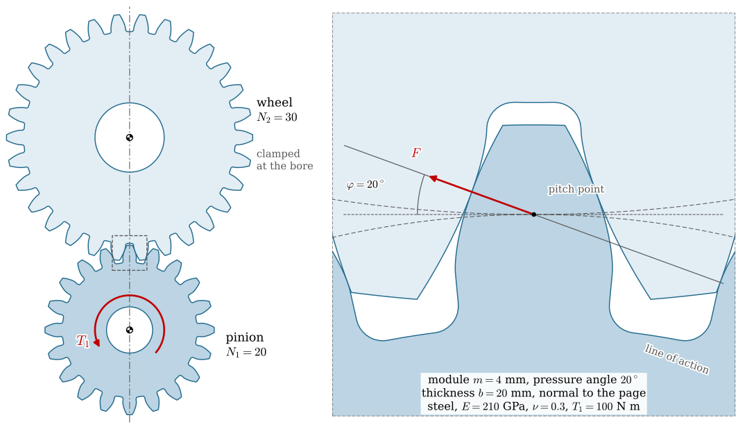
A pinion of \(N_1 = 20\) teeth drives a wheel of \(N_2 = 30\), module \(m = 4\) mm, pressure angle \(20°\), both of steel, \(E = 210\) GPa and \(\nu = 0.3\), and the gears are \(b = 20\) mm thick (Figure 9.4.6). The pinion torque is \(T_1 = 100\) N·m. Find the tooth forces, the contact ratio and the Lewis stresses, then compute the stress in the teeth with the finite element method as the gears turn through the mesh, and compare.
Figure 9.4.6: The gears of Example 5, and the teeth at the pitch point zoomed. The tooth force \(F\) acts along the line of action at the pressure angle; the gears are \(b = 20\) mm thick, normal to the page, and the model treats them as plane bodies of that thickness.
The forces from 9.4.12, the contact ratio from 9.4.15 and the Lewis stresses from 9.4.13 are
\[ \begin{aligned}F_t &=2500.0~\text{N},\quad F_r =909.9~\text{N},\quad F =2660.0~\text{N}\\ L &=18.95~\text{mm},\quad p_b =11.81~\text{mm},\quad \varepsilon =1.605\\ \sigma_1 &=97.05~\text{MPa},\quad \sigma_2 =87.05~\text{MPa}\end{aligned} \]
The finite element model treats each gear as a plane body of thickness \(b\) in plane stress, clamped at its bore, which takes up the torque as a shaft would. Its displacement \(\bm u\) satisfies the weak form of elastostatics of the Gridap chapters,
\[
\int_\Omega \bm\varepsilon(\bm v) : \bm\sigma(\bm u)\, d\Omega
= \int_\Gamma \bm v \cdot \bm t \, d\Gamma
\quad \text{for all } \bm v
\tag{9.4.16}\]
where the traction \(\bm t\) on the tooth outline \(\Gamma\) is the tooth force. The model does not solve the contact between the teeth; it applies the force where the involute theory puts it. For a pinion angle \(\theta_1\), the contact points lie on the line of action one base pitch apart, and each pair whose point lies between the addendum circles carries \(F\), or \(F/2\) when two pairs are in contact, along the line of action. On each flank the force is spread as a semi-elliptic pressure over a strip of half-width \(a_s = 0.4\) mm,
the shape of a Hertz contact pressure, with \(s\) along the flank.
The width of the strip is our choice, and the true contact area is not. Near the point of contact each involute flank is close to a circle whose radius is the involute’s radius of curvature, the distance along the line of action from the contact point to the point where the line touches that gear’s base circle. At the pitch point this is \(\rho = r\sin\varphi\), and elsewhere \(\rho_1 = r_{b1}\tan\varphi + s\) and \(\rho_2 = r_{b2}\tan\varphi - s\) for a contact at the distance \(s\) from the pitch point. Two elastic cylinders pressed together touch over a strip whose width Hertz’s theory gives. Following [1, Eqs. 3-73 and 14-10], for two steel teeth with the same \(E\) and \(\nu\), the half-width of the strip and the largest pressure in it are
\[
a = \sqrt{\frac{8F(1 - \nu^2)}{\pi b E}\,\frac{\rho_1\rho_2}{\rho_1 + \rho_2}},
\qquad p_\text{max} = \frac{2F}{\pi a b}
\tag{9.4.18}\]
At the pitch point of Example 5, where one pair carries the whole force,
The contact is a strip about a fifth of a millimetre wide across the whole face of the tooth, less than a quarter of the strip in the model, and its pressure is more than three times higher. Resolving it would take elements of a few hundredths of a millimetre at every contact point and a contact algorithm, and the result is known anyway from 9.4.18: this is the contact stress against which a hardened flank is rated for pitting. The model therefore shows the contact peak too low on purpose. The stress at the root, a tooth height away, does not depend on how the force is spread, by Saint-Venant’s principle. Splitting the force equally in double contact ignores that the two pairs are not equally stiff, which makes the load on each pair vary along the stretch.
The gears are meshed with triangles of 0.1 mm along the whole outline, fine enough to resolve the root fillet of radius \(0.3m\): refining further changes the root stress by less than 0.1 %. With quadratic elements the pinion has 350 000 degrees of freedom and the wheel 530 000. The stiffness matrix does not change as the gears turn, only the load does, so each gear’s matrix is assembled and factorized once and every one of the 120 positions of Figure 9.4.7 costs only a new right-hand side and a back substitution. The heart of the script Gridap/gears/gears.jl is
A =assemble_matrix((u, v) ->∫(ε(v) ⊙ (σ∘ε(u)))dΩ, U, V)K =lu(A) # once per gearfor θ1in θs # 120 positions of the pinion t =traction(θ1) # strips at the contact points of θ1 rhs =assemble_vector(v ->∫(v ⋅ t)dΓ, V) uh =FEFunction(U, K \ rhs) # a back substitution per frameend
and the whole run, meshing, factorization and 240 solutions, takes about five minutes.
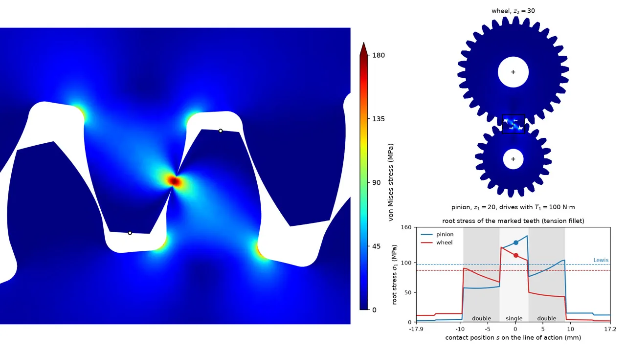
Figure 9.4.7: Von Mises stress in the gears of Example 5 as the pinion (below) drives the wheel (above) through three teeth. Left: the meshing zone. Top right: the whole pair. Bottom right: the largest principal stress in the tension fillet of the two marked teeth against the position \(s\) of their contact on the line of action, with the zones of double and single contact and the Lewis stresses as dashed lines.
The model is plane linear elasticity in Gridap [2,3], plane stress, for each gear separately; the scripts are outlines.py, which writes the tooth outlines with a root fillet of \(0.3m\), gears.jl, which meshes and solves, and render.py, which draws the frames.
pinion
wheel
elements
83 962
126 757
degrees of freedom
349 694
527 436
Mesh: triangles from gmsh, 0.10 mm along the whole tooth outline, growing to 2 mm from 6 mm inside it; displacements interpolated with quadratic (six-node) Lagrange elements. Refining to 0.07 mm changes the root stress by less than 0.1 %.
Boundary conditions: the bore (diameter \(0.3d\)) clamped, \(\bm u = \bm 0\).
Load: no contact is solved. At each of the 120 positions the force of each pair in contact acts along the line of action at the point where the involutes cross it, spread over a semi-elliptic strip of half-width 0.4 mm; two pairs in contact share it equally. The centre distance is 0.2 mm larger than standard so that the idle flanks do not touch.
Solution: the stiffness matrix of each gear is assembled and LU-factorized once, about 50 s; each position then costs a new load vector and a back substitution, about 2 s for both gears. Stresses are averaged from the elements to the nodes.
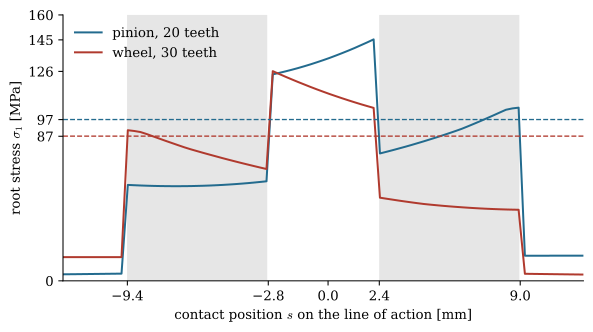
The tooth pairs of Figure 9.4.7 run through the same cycle. A pair comes into contact at the pinion’s root and the wheel’s tip while the pair ahead still carries half the load. When that pair leaves, the whole force jumps onto the new pair, and its root stresses double. In the middle of the stretch the pair carries the load alone, the wheel’s root stress falling and the pinion’s rising as the contact climbs the pinion tooth, until the next pair arrives and takes half. Figure 9.4.8 reads the root stresses of the marked teeth from the results.
Figure 9.4.8: Largest principal stress in the tension fillet of a pinion tooth and a wheel tooth over one passage through the mesh, from the finite element model, against the Lewis estimate (dashed). The grey bands are the double-contact zones.
In single contact the finite element stresses exceed Lewis’s by about half:
Two effects pull in opposite directions. Lewis puts the force at the tip, but the single pair never carries it there: the second pair takes half the load before the contact reaches the tip, so the largest moment arm in single contact is shorter than Lewis assumes. The fillet, which Lewis treats as a smooth beam, concentrates the stress, and that wins: most of the factor of about 1.5 is the stress concentration of the root fillet of radius \(0.3m\). Lewis’s equation is a sound way to size a gear’s module and face width, provided its allowable stress has room for this factor. The model also shows a stress that Lewis leaves out: the opposite fillet of each tooth is in compression, and its von Mises stress is even higher, up to 170 MPa on the pinion, because the radial component of the force adds to the bending there. Gear teeth fail in fatigue from the fillet in tension, where cracks open.
Load variation in spur and helical gears
The root stress of Figure 9.4.8 follows the force on one tooth, and that force jumps whenever a pair of teeth comes into or out of contact. The graph of the force on one tooth over its passage through the mesh is the load variationsv. kraftvariation of the gear pair, and here helical gears differ from spur gears.
Figure 9.4.9: The gears of Example 5 as helical gears, helix angle \(20°\), the pinion right-hand and the wheel left-hand. Each tooth comes into mesh at one face and the contact travels across the face width as the gears turn.
All contacts of a gear pair lie in the plane of action, the plane through the line of action and parallel to the axes. The part of it where the teeth can touch is a rectangle, the length of action \(L\) of 9.4.14 long and the face width \(b\) wide. A spur tooth touches its mate along a line across the whole face, parallel to the axes, and the lines of successive teeth follow each other along the rectangle one base pitch \(p_b\) apart. A helical tooth (Figure 9.4.9) touches along a line inclined at the base helix angle\(\beta_b\), \(\tan\beta_b = \tan\beta\cos\varphi\), so its line enters the rectangle at one corner, grows as the gears turn, and leaves the opposite corner as gradually as it came. A cut through a helical gear across its thickness shows why. Every section is the spur outline, turned a little further by the helix the deeper the cut; a cut at any depth therefore shows a spur gear pair in mesh, and its contact points lie on the line of action. Moving the cut through the thickness turns the sections, and the contact points slide along the line of action: together they trace the inclined contact lines of Figure 9.4.10.
Figure 9.4.10: The pinion of Figure 9.4.9 cut at a depth \(z\) that moves through its thickness, the gears standing still. The section (hatched) and the wheel’s section in the same plane (black outline) are a spur gear pair; the red dots are their contact points. Below the cut, the red lines are the contact lines across the pinion’s flanks. Right: the plane of action seen face on, where the contact lines are straight and inclined, and the cut meets them at the contact points of the section.
A contact line spans \(b\tan\beta_b\) along the line of action, and that, in base pitches, adds the overlap ratio to the contact ratio,
the total contact ratio, the mean number of teeth in contact.
To turn the contact lines into forces we assume that the teeth are equally stiff along the lines, so that the force per unit length of contact line is the same on all of them. A tooth whose line has the length \(\ell_k\) inside the rectangle then carries the share
of the force, where \(s_k\) is the position of the line at mid-face, the bracket is one where the line is inside the rectangle and zero elsewhere, and the line of the next tooth lies at \(s_k + p_b\). For a spur gear, \(\beta_b = 0\), each line is in or out as a whole, and 9.4.20 reduces to the equal split of Example 5.
Code
s_a0 =-np.sqrt((r_2 + m_g)**2- (r_2*np.cos(phi))**2) + r_2*np.sin(phi) # wheel's tips_r0 = np.sqrt((r_1 + m_g)**2- (r_1*np.cos(phi))**2) - r_1*np.sin(phi) # pinion's tipz = np.linspace(-b_g/2, b_g/2, 2001)def load_share(beta_deg, s):# share of the force on the tooth whose contact line is at s (mid-face), eq-tr-load-share tb = np.tan(np.radians(beta_deg))*np.cos(phi)def length(sk): # the part of the line inside the rectangle inside = (s_a0 <= sk[:, None] + z*tb) & (sk[:, None] + z*tb <= s_r0)return inside.mean(axis=1)*b_g*np.sqrt(1+ tb**2) total =sum(length(s + k*p_b) for k inrange(-4, 5))return length(s)/total, b_g*tb/p_bs_line = np.linspace(s_a0 -12, s_r0 +12, 1500)share_spur, _ = load_share(0, s_line)share_hel, eps_beta = load_share(20, s_line)
Code
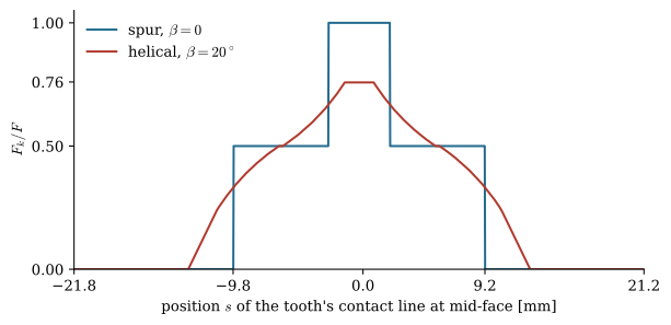
fig, ax = plt.subplots(figsize=(7, 3.2))ax.plot(s_line, share_spur, color=BLUE, label=r'spur, $\beta = 0$')ax.plot(s_line, share_hel, color=RED, label=r'helical, $\beta = 20^\circ$')ax.set_xlim(s_line[0], s_line[-1])ax.set_ylim(0, 1.05)ax.set_xticks([round(s_line[0], 1), round(s_a0, 1), 0, round(s_r0, 1), round(s_line[-1], 1)])ax.set_yticks([0, 0.5, round(share_hel.max(), 2), 1])ax.set_xlabel('position $s$ of the tooth\'s contact line at mid-face [mm]')ax.set_ylabel('$F_k/F$')ax.legend(loc='upper left', frameon=False)for side in ('top', 'right'): ax.spines[side].set_visible(False)plt.show()
Figure 9.4.11: The load variationsv. kraftvariation of one tooth of the gears of Example 5 as spur gears and as helical gears with \(\beta = 20°\) and the same transverse geometry, from 9.4.20: the share of the tooth force \(F\) that the tooth carries as its contact line passes through the plane of action.
The spur tooth of Figure 9.4.11 takes half the force at once, all of it a moment later, then half again, and lets go of it at once: every step is a jump in the deflection of the teeth, which the gears hear as a knock and the drive as a vibration at the tooth frequency. The helical tooth takes its load up and puts it down gradually, the total length of contact line hardly changes as the gears turn, and the largest share of a tooth is well below the whole force. Helical gears therefore run more quietly and carry more load for the same size; the axial force is the price, and the herringbone gear removes it. The assumption of equal stiffness per unit length is the weak point of 9.4.20: a line near the tip of a tooth meets a softer tooth than one near the root, and the rating standards correct for this with load distribution factors.
The load diagram
A gear supplier’s catalogue answers the designer’s first question, how much torque a gear of a given module and number of teeth can carry, with a load diagramsv. belastningsdiagram: the torque against the number of teeth on logarithmic axes, one line per module. We now build one from the two limits of this section, the bending stress at the root and the contact pressure on the flank, and check it against the load diagrams of a Swedish supplier’s catalogue [4].
The flank limit follows from 9.4.18. At the pitch point the radii of curvature are \(\rho_1 = (d_1/2)\sin\varphi\) and \(\rho_2 = u\rho_1\), where \(u = N_2/N_1\) is the gear ratio, and the tooth force is \(F = 2T/(d_1\cos\varphi)\). Inserting these and requiring the largest pressure to stay below the allowable flank pressure \(\sigma_{HP}\) gives the torque the flank carries:
Code
T, d_1, u, b, phi_s, E_s, nu_s, sig_HP = sp.symbols(r'T d_1 u b varphi E nu sigma_HP', positive=True)rho_1 = d_1/2*sp.sin(phi_s)rho_2 = u*rho_1F_n =2*T/(d_1*sp.cos(phi_s))a_h = sp.sqrt(8*F_n*(1- nu_s**2)/(sp.pi*b*E_s)*rho_1*rho_2/(rho_1 + rho_2)) # eq-tr-hertzp_max =2*F_n/(sp.pi*a_h*b)T_H = sp.solve(sp.Eq(p_max**2, sig_HP**2), T)[0]Z_E2, Z_H2 = E_s/(2*sp.pi*(1- nu_s**2)), 2/(sp.sin(phi_s)*sp.cos(phi_s))check = sp.simplify(T_H - sig_HP**2*b*d_1**2*u/(2*Z_E2*Z_H2*(u +1))) # zero: the ISO form
\[ T_H =\dfrac{\pi b d_{1}^{2} \sigma_{HP}^{2} u \left(1 - \nu^{2}\right) \sin{\left(2 \varphi \right)}}{4 E \left(u + 1\right)} \]
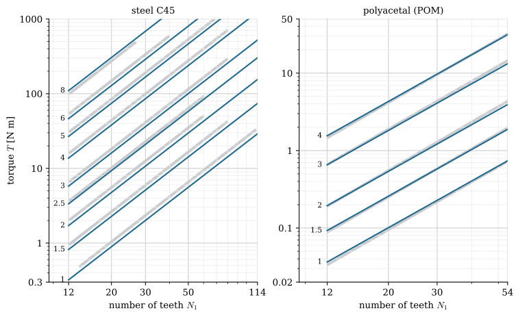
In the notation of ISO 6336 this is \(T_H = \sigma_{HP}^2\, b\, d_1^2\, u/(2 Z_E^2 Z_H^2 (u + 1))\), with the elasticity factor\(Z_E = \sqrt{E/(2\pi(1 - \nu^2))}\) and the zone factor\(Z_H = \sqrt{2/(\sin\varphi\cos\varphi)}\); the code above checks that the two forms agree. The root limit follows from Lewis’s equation 9.4.13 with the fillet’s stress concentration \(K_t\) that Example 5 measured and the allowable local root stress \(\sigma_{FP}\). With \(d_1 = mN_1\) the two limits are, as mechanicskit.gears computes them,
and the gear carries the smaller of the two. On logarithmic axes both are straight lines for each module: the flank limit rises with the square of the number of teeth, slope 2, because a larger gear has flatter flanks that spread the contact; the root limit rises only as \(N_1 Y\), a slope of about 1.3. Depending on the material, the flank or the root governs.
For the steel, the catalogue’s C45 is close to AISI 1045, which has a hardness of 163 HB hot-rolled and 179 HB cold-drawn [1, Table A-20]. HB is the Brinell hardness: a hard ball is pressed into the surface with a known force, and the force divided by the area of the dent it leaves, in kgf/mm², is the hardness. A harder steel resists the local yielding under a contact, and its ultimate strength is roughly \(3.4\,\text{HB}\) MPa [1], so hardness stands in for strength in the rating standards. For normalised steel, according to ISO 6336-5 [5], the allowable stresses are straight lines in the hardness, \(\sigma_{H\lim} = \text{HB} + 190\) MPa and \(\sigma_{F\lim} = 0.455\,\text{HB} + 69\) MPa for the usual material quality. Here \(\sigma_{F\lim}\) is a nominal root stress that already contains a stress concentration of 2, so the local stress the material bears is \(2\sigma_{F\lim}\). The catalogue states its safety factors, 1.0 on the flank and 1.4 on the root, its face widths, and that its torques hold for the smaller gear; we take \(u = 1\), equal gears, where the flank pressure is highest. For the plastic gears, polyacetal (POM) with \(E = 3100\) MPa and \(\nu = 0.35\)[6], we found no reliable published allowable flank pressure, so we fit it to the catalogue’s plastic diagram. For the root of POM, according to VDI 2736 as quoted by Bae and Kissling [7,8], the fatigue strength is 41 MPa for \(10^7\) cycles at 20 °C, which we treat like \(\sigma_{F\lim}\) for steel.
Code
from mechanicskit.gears import flank_torque, root_torque, iso6336_normalisedcat = pd.read_csv('data/load_diagram_mekanex.csv', comment='#')K_t = sig_fe1/sig_L1 # fillet stress concentration, from Example 5def limits(N, m, b, mat):# torques [N m] that the flank and the root carry, eq-tr-load-limitsreturn (flank_torque(N, m, b, mat['sig_HP'], mat['E'], mat['nu']), root_torque(N, m, b, mat['sig_FP'], K_t))s_Hlim, s_FE = iso6336_normalised(179) # AISI 1045 cold drawn, 179 HBsteel =dict(E=210e3, nu=0.3, sig_HP=s_Hlim/1.0, sig_FP=s_FE/1.4, widths={1: 15, 1.5: 17, 2: 20, 2.5: 25, 3: 30, 4: 40, 5: 50, 6: 60, 8: 80})pom =dict(E=3100.0, nu=0.35, sig_HP=1.0, sig_FP=2*41/1.4, widths={1: 15, 1.5: 17, 2: 20, 3: 30, 4: 40})def catalogue_ratio(material, mat):# catalogue torque over model flank torque, at both ends of every digitised line r = []for _, row in cat[cat.material == material].iterrows():for N, T_c in ((row.N_start, row.T_start_Nm), (row.N_end, row.T_end_Nm)): r.append(T_c/limits(N, row.module, mat['widths'][row.module], mat)[0])return np.array(r)r_steel = catalogue_ratio('steel', steel)pom['sig_HP'] = np.sqrt(np.median(catalogue_ratio('plastic', pom))) # fitted, from sigma_HP = 1r_pom = catalogue_ratio('plastic', pom)
With these values the steel model and the plastic fit give
Figure 9.4.12: The load diagramsv. belastningsdiagram from 9.4.21, one line per module (the number at its left end), for steel and for polyacetal gears with the catalogue’s face widths and \(u = 1\) (blue), over the lines of the catalogue’s load diagrams [4] (grey). The flank limit governs every line.
The steel model reproduces the catalogue’s diagram from first principles: the slope of 2, which the catalogue lines have to three digits, and the torques to within the ratio above, about 15 % below the catalogue. The difference is the hardness. The catalogue’s lines match \(\sigma_{HP} \approx 400\) MPa, which ISO 6336-5 gives normalised steel of 210 HB, the top of its range and harder than the cold-drawn 1045 of Shigley’s table. The module 8 line of the catalogue lies 20 % below the others, which no factor in 9.4.21 explains, so we take it for a drawing error. The root never governs a steel gear of this kind: even with 114 teeth the root carries several times the torque the flank does.
The catalogue’s plastic lines also have slope 2, so they too are a flank limit, and fitting them gives the allowable flank pressure of POM above, about 15 MPa. Polyacetal gears that run dry wear and heat up, and the teeth soften as they warm, long before the root breaks: the root limit of 9.4.21, from VDI 2736’s fatigue strength, lies far above the catalogue’s lines. VDI 2736 therefore checks plastic gears for temperature and wear as well as for stress.
For gears printed by fused-filament fabrication we cannot draw such a diagram yet. Their strength depends on the polymer, on the orientation of the layers relative to the tooth, on how well the layers are fused, and on the temperature the teeth reach in running, and neither VDI 2736 nor the published tests cover the filaments and settings we print with. The diagram for printed gears has to come from mechanical testing: fatigue tests of printed teeth in the orientations we print, and running tests of gear pairs at known torque and speed that measure wear and tooth temperature. 9.4.21 then needs only the two allowable stresses those tests give.
The notebook below draws the load diagram for any material hardness, face width, gear ratio and safety factors, and shows which limit governs a chosen gear.
TipIn industry: gear rating standards and catalogues
Nobody sizes a production gearbox with Lewis’s equation alone. ISO 6336 and AGMA 2001 compute the root stress from the Lewis form with a form factor taken at the highest point of single contact, a stress correction factor for the fillet, a load sharing factor from the contact ratio, and factors for the dynamic load, the uneven load across the face width and the type of driving and driven machine. They also rate the flanks for pitting from the Hertz contact stress, which the model of Example 5 smeared out on purpose; pitting, not tooth breakage, usually limits a hardened gear. Software such as KISSsoft does the calculation. A machine builder rarely designs gears at all, and selects a geared motor from a catalogue instead, by its output speed and torque times a service factor, 1.0 for a smooth load eight hours a day and up to 2 for heavy shocks around the clock.
Towards a contact model
The model of Example 5 places the tooth forces where the involute theory says they act, spreads them over a strip of our choosing, and splits them equally between two pairs of teeth. Each of these three shortcuts can be replaced by mechanics. This section takes the first step towards a model that finds the contact itself: we solve a true contact problem for the simplest case, check it against Hertz, and then use what it confirms to give the gear model the true contact strips and a load sharing that follows from the stiffness of the teeth. The scripts are in Gridap/gears/ (hertz_cylinder.jl, gears_hertz.jl).
Contact solved: a cylinder on a plane
A contact condition says that two bodies may touch but not overlap, and that the surfaces push and never pull. Let \(g = y + u_y\) be the gap between a point of a steel cylinder’s surface and a rigid plane at \(y = 0\): the point may not go below the plane, \(g \ge 0\), and the plane pushes on it only where it touches. The penalty method replaces this condition by a stiff spring that acts only on overlap, the traction \(t_y = \kappa\langle -g\rangle\) with \(\langle x\rangle = \max(0, x)\), and adds its work to the weak form of the cylinder,
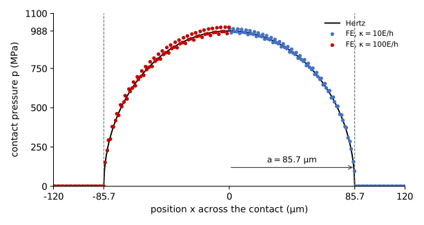
The bracket makes the problem nonlinear, since where the contact ends depends on the solution, and Newton’s method solves it. A large penalty \(\kappa\) allows only a tiny overlap, and the answer stops changing once \(\kappa\) is large enough: going from \(\kappa = 10E/h\) to \(100E/h\), with \(h\) the element size at the contact, moves the results by 0.1 to 0.3 %. The cylinder has \(R = 10\) mm and carries 133 N per mm of length, the tooth force of Example 5 per millimetre of face width, in plane strain; a quarter of it is meshed with elements of 2.9 µm at the contact, a thirtieth of the contact half-width.
finite elements
Hertz
half-width \(a\) [µm]
85.7
85.7
largest pressure \(p_\max\) [MPa]
989
988
largest von Mises stress [MPa]
553
551
its depth [µm]
61
60
largest shear stress [MPa]
298
297
its depth [µm]
68
67
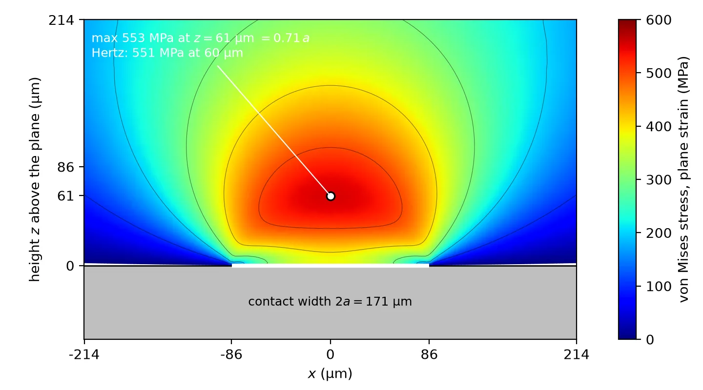
The contact model and Hertz’s theory agree to within a fraction of a percent (Figure 9.4.13). The pressure has the semi-elliptic shape that 9.4.18 assumes, and the largest stress is not at the surface but 0.7 half-widths below it, where the pressure from above and the support from the sides combine into the largest shear. This is where pitting starts: a crack grows from below the surface, parallel to it, until a flake of the flank breaks out. According to [1], the largest shear stress of a cylinder contact is \(0.30\,p_\max\) at the depth \(0.786a\), which the model reproduces.
(a) The contact pressure from the penalty model with two penalty stiffnesses (dots), on the Hertz ellipse (line).
(b) The von Mises stress below the contact, with its maximum below the surface.
Figure 9.4.13: A steel cylinder of radius 10 mm pressed on a rigid plane with 133 N/mm, solved as a contact problem with the penalty method in Gridap, against Hertz’s theory.
This is the one true contact problem of the chapter: where the cylinder touches the plane is part of the solution. The script is hertz_cylinder.jl, the plots hertz_plots.py.
Model: a quarter of the cylinder, \(R = 10\) mm, plane strain, with symmetry (\(u_x = 0\)) on the vertical cut and the displacement prescribed on the horizontal cut; a secant iteration on that displacement makes the contact force 133.0 N/mm.
Mesh: 11 545 triangles, 46 390 degrees of freedom, quadratic Lagrange elements; 2.9 µm at the contact, a thirtieth of the half-width, graded outwards.
Contact: the penalty traction of 9.4.22 with \(\kappa = 10E/h\) and, as a check, \(100E/h\), solved by Newton’s method with a backtracking line search (17 steps).
Run time about two minutes on one CPU.
True contact strips and load sharing in the gears
With the contact model confirming 9.4.18, the gear model can take its strips from it. At each contact point the radii of curvature are the distances along the line of action to the two tangent points of the base circles, and the force of the pair then gives the half-width \(a\) and the pressure of 9.4.18. Resolving strips about 0.1 mm wide takes elements of 12.5 µm along the flanks of the teeth that pass through the mesh, about 0.8 million degrees of freedom in the pinion and 1.1 million in the wheel; the stiffness is still factorized once.
The equal split in double contact goes next. Two pairs of teeth in contact must close the same gap: the gears are rigid bodies apart from the deformation of the teeth, so both pairs approach by the same amount \(\delta_0\) as the torque winds the gears up. Let \(C_{ij}\) be the approach of pair \(i\), the movement of the two flanks towards each other along the line of action, under a unit force on pair \(j\); the model computes it with two extra back substitutions per gear. The forces \(f_1, f_2\) on the two pairs then satisfy
\[
\bm C \bm f = \delta_0 \begin{bmatrix} 1 \\ 1 \end{bmatrix}, \qquad f_1 + f_2 = F
\quad\Rightarrow\quad
\bm f = F\,\frac{\bm C^{-1}\bm 1}{\bm 1^{\mathsf{T}}\bm C^{-1}\bm 1}
\tag{9.4.23}\]
and the mesh stiffness\(k = F/\delta_0\) is the stiffness of the whole mesh against the torque. Since \(a\) depends on the force and the compliance weakly on \(a\), two or three passes settle each frame.
Figure 9.4.14: The gears of Example 5 with the true Hertz strips and the load shared by stiffness. The contact is still not solved: the strips are placed and sized by Hertz’s theory, which Figure 9.4.13 has just confirmed. Left: a window 0.6 mm wide on the contact of the marked pair, with the largest von Mises stress below each flank (circles). Top right: the meshing zone on a logarithmic scale, so that the roots and the contacts both show. Bottom right: the share of the force that a pair carries, from the stiffness and from the equal split.
The same plane-stress model as Figure 9.4.7, with two changes: the strips have the Hertz half-width and pressure of each pair’s force, and the force is shared by the stiffness of the pairs, 9.4.23. The scripts are gears_hertz.jl, render_hertz.py and share_plots.py.
pinion
wheel
elements
197 276
258 943
degrees of freedom
809 228
1 063 538
Mesh: triangles of 12.5 µm (a ninth of the Hertz half-width) within 0.15 mm of the loaded flanks of the five teeth that pass through the mesh (pinion teeth 0, 1, 2, 18, 19; wheel teeth 0, 1, 2, 28, 29), growing to 0.1 mm at 0.6 mm and to 2 mm in the body; quadratic Lagrange elements. The involutes are resampled every 0.01 mm of arc length.
Load: at each of the 120 positions, Hertz strips at the contact points, with the half-width from the radii of curvature \(\rho_1 = r_{b1}\tan\varphi_w + s\) and \(\rho_2 = r_{b2}\tan\varphi_w - s\); the Hertz formula is that of plane strain, the model plane stress.
Load sharing: in double contact the compliance matrix \(\bm C\) is found with unit strip loads, then the shares and the half-widths are iterated, two or three passes per frame.
Solution: one LU factorization per gear (80 s), then back substitutions only; 120 frames in about 17 minutes. The von Mises stress uses \(\sigma_{zz} = \nu(\sigma_{xx} + \sigma_{yy})\), the plane-strain state under the contact.
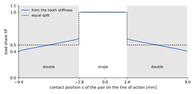
(a) The share of the tooth force a pair carries, from the tooth stiffness against the equal split.
(b) The mesh stiffness, per millimetre of face width.
Figure 9.4.15: The load variation of the spur gears of Example 5 from the stiffness of the teeth, and the mesh stiffness over one passage of a pair through the mesh.
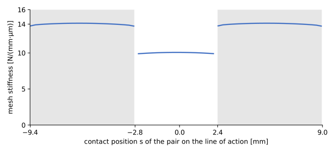
At the pitch point the gear model reproduces the cylinder: a half-width of 0.111 mm, a Hertz pressure of 765 MPa, and the largest von Mises stress, 440 MPa or 0.575 of the pressure, 0.69 half-widths below the flank, within 3 % of the theory with elements a ninth of the half-width. The load sharing of Figure 9.4.15 differs from the equal split: a pair that enters takes only 40 % of the force, because its contact is at the wheel’s tip and the pinion’s root, where the wheel’s tooth is most flexible, and its share grows to 60 % as the contact moves towards the pitch point. The load variationsv. kraftvariation of a spur pair is therefore not a staircase but a ramp with two steps, and the root stress in double contact is up to 19 % lower than with the equal split. The largest root stress, in single contact, does not change, so the conclusions of Example 5 stand. The mesh stiffness jumps between about 10 and 14 N/(mm·µm) each time a pair enters or leaves; the gears deflect a little more and a little less at the tooth frequency, and that periodic deflection excites the whine of spur gears.
What remains is a contact model of the gears themselves, with the penalty condition of 9.4.22 between the two flanks instead of the prescribed strips. That needs the gap between two separately meshed bodies, which Gridap does not provide, and a nonlinear solution for every frame. It would find the contact points, the strips and the load sharing at once, including the edge contacts at the tips that the prescribed strips can only approximate, and it is the next model for the Gridap part of this book.
Problems
Problem 1: A different idler. The middle gear of Figure 9.4.16 is replaced by one with 60 teeth, and the shafts of the outer gears are moved apart to keep the mesh. What are the new output speed and torque, and the load on the idler’s pin? What happens if the idler is removed and the left gear drives the right gear directly?
Figure 9.4.16: The gear train of Problem 1, as in Example 1.
Answer:The idler cancels: \(n_3 = 1450 \cdot 24/16 = 2175\) rpm and \(T_3 = 6.59\) N·m as before, and the pin still carries \(2F_t = 549\) N. Without the idler the output turns at the same speed in the opposite direction.
Problem 2: Self-locking. The worm drive of Figure 9.4.17 is to hold a load with the motor off. With \(q = 10\), \(\varphi = 20°\) and \(f = 0.05\), what is the largest lead angle and the largest number of starts that make it self-locking? What would \(q\) have to be for a single-start worm, and what is the forward efficiency then?
Figure 9.4.17: The worm drive of Problem 2.
Answer:Self-locking needs \(\tan\lambda \le f/\cos\varphi_n \approx 0.053\), \(\lambda \le 3.0°\). No number of starts reaches that with \(q = 10\) (one start gives \(5.7°\)). A single start needs \(q \ge 19\), and then \(\eta = (0.94 - 0.05 \cdot 0.053)/(0.94 + 0.05 \cdot 19) \approx 0.50\).
Problem 3: A bevel gear for a differential. The bevel pair of Figure 9.4.18 is redesigned for a ratio of 4 with a 13-tooth pinion. Find the wheel’s number of teeth, the cone angles and the pinion’s virtual number of teeth. Does the pinion need a profile shift?
Figure 9.4.18: The bevel gear pair of Problem 3.
Answer:\(N_2 = 52\), \(\delta_1 = \arctan(1/4) = 14.0°\), \(\delta_2 = 76.0°\), \(N_{v1} = 13/\cos 14.0° = 13.4 < 17\): yes, without it the pinion is undercut.
Problem 4: Sizing by Lewis. The gears of Figure 9.4.19 are to carry \(T_1 = 250\) N·m with the same teeth, \(N_1 = 20\) and \(N_2 = 30\). The steel allows 190 MPa in bending at the root, and the finite element results of Example 5 show that the true root stress is about 1.5 times Lewis’s. Which module is needed with \(b = 10m\)?
Figure 9.4.19: The gear pair of Problem 4.
Answer:\(F_t = 2T_1/(mN_1)\) and \(\sigma = 1.5\,F_t/(b m Y) = 1.5 \cdot 2T_1/(10\,m^3 N_1
Y) \le 190\) MPa give \(m^3 \ge 1.5 \cdot 2 \cdot 250 \cdot 10^3/(10 \cdot 20 \cdot 0.322
\cdot 190) = 61.3\) mm³, \(m \ge 3.94\) mm: module 4 with \(b = 40\) mm.
Problem 5: One wheel on a wet floor. The RC car of Example 4 stands with its left rear wheel on a wet tile, where friction lets the wheel take at most 0.05 N·m, and its right rear wheel on carpet, good for 0.8 N·m. How much torque can the rear axle put on the ground with the open differential of Figure 9.4.20, and how much with the differential locked? What does the left wheel do when the motor gives more?
Figure 9.4.20: The differential of Problem 5.
Answer:Open: both wheels get the same torque, at most 0.05 N·m, so the axle delivers 0.1 N·m, and any more torque spins the left wheel while the right one stops. Locked: the wheels turn together and each takes what its grip allows, \(0.05 + 0.8 = 0.85\) N·m.
Further reading
Budynas and Nisbett [1, Chs. 13 and 14] cover the kinematics, forces and efficiency of spur, helical, bevel and worm gears, and Lewis’s equation with the AGMA corrections that turn it into a rating method. Björk [9] gives the ISO formulas for gear geometry and strength in the form Swedish engineers look them up. The finite element model of Example 5 is written in Gridap [2,3], like the torsion model of the Gridap part.
Badia S, Verdugo F. Gridap: An extensible finite element toolbox in Julia. Journal of Open Source Software 2020;5:2520. https://doi.org/10.21105/joss.02520.
[3]
Verdugo F, Badia S. The software design of Gridap: A finite element package based on the JuliaJIT compiler. Computer Physics Communications 2022;276:108341. https://doi.org/10.1016/j.cpc.2022.108341.
ISO 6336-5:2016 Calculation of load capacity of spur and helical gears – Part 5: Strength and quality of materials. Geneva, Switzerland: International Organization for Standardization; 2016.
[6]
Tavčar J, Černe B, Duhovnik J, Zorko D. A multicriteria function for polymer gear design optimization. Journal of Computational Design and Engineering 2021;8:581–99. https://doi.org/10.1093/jcde/qwaa097.
[7]
VDI 2736 Blatt 2: Thermoplastische Zahnräder – Stirnradgetriebe – Tragfähigkeitsberechnung. Berlin: Verein Deutscher Ingenieure; Beuth; 2014.