A motor drives a pump, a gearbox drives a wheel, a tractor drives a mower behind it, and in each case two shafts that were made and mounted separately have to turn together. A shaft couplingsv. axelkoppling joins them. If the two shafts lay on one line, a sleeve bolted to both would do, but they never do: the motor sits on its own feet, the bearings have play, the frame bends under load, and a car’s wheel moves up and down with the suspension and turns with the steering. Most of what a coupling does is to carry the torque while it allows the shafts to be out of line.
This chapter starts from the ways two shafts can be out of line and the rigid coupling that allows none of them. It then takes the couplings that allow some misalignment by giving way (the jaw coupling with its elastic spider) or by sliding (the Oldham coupling), the Schmidt coupling for large parallel offsets, and the Hooke jointsv. kardanknut, whose output does not turn at the speed of its input. Two Hooke joints can cancel each other’s error, and the ball joints of a car’s drive shafts avoid it altogether; the RC car of the course needs them at its front wheels. The last part is the splinesv. bomförband: it carries the torque into a hub and lets the hub slide along the shaft as the drive shaft changes length.
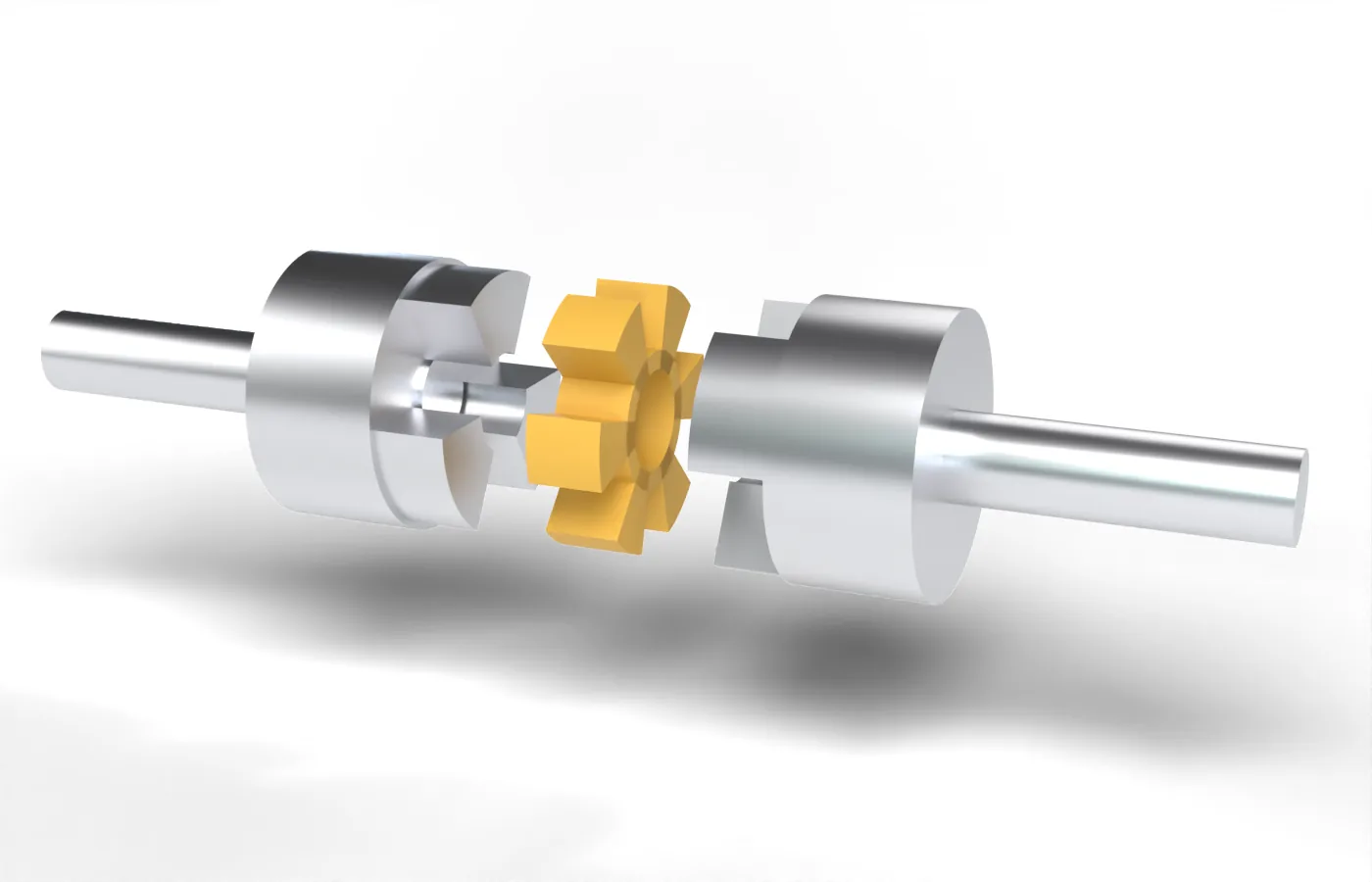
Figure 9.14.1: A jaw coupling pulled apart: two hubs with three jaws each and the elastic spider that sits between them.
Shafts out of line
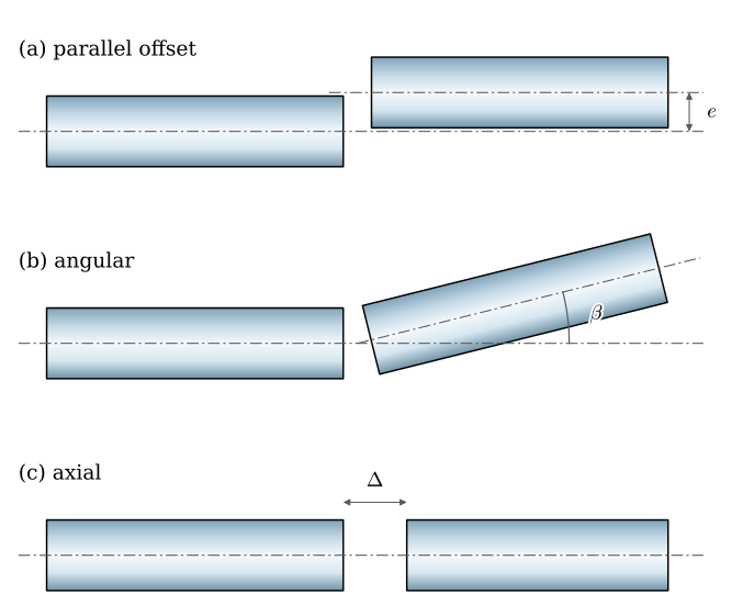
Two shafts can be out of line in three ways (Figure 9.14.2). Their axes can be parallel but offset by \(e\), they can meet at an angle \(\beta\), or the gap between the shaft ends can change by \(\Delta\), as when a shaft grows with temperature or a drive shaft swings with the suspension. A real pair of shafts has all three at once, and the misalignmentsv. uppriktningsfel a coupling has to take is their combination.
Figure 9.14.2: The three kinds of misalignment: (a) parallel offset \(e\), (b) angle \(\beta\) between the axes, (c) a change \(\Delta\) in the axial gap.
A coupling that does not allow a misalignment forces the shafts into line, and the force it takes to do that goes into the bearings. A steel shaft of 40 mm diameter, held in line by its bearings over 300 mm and pushed sideways by 0.1 mm at the other end, bends like a beam clamped at one end and guided at the other, with the stiffness \(12EI/L^3\): about 1 kN for that tenth of a millimetre. The force turns with the shaft, so the bearings and the shaft see it as a load that reverses every revolution: a fatigue load. A coupling is either rigid, and then the shafts are aligned to a few hundredths of a millimetre when they are mounted, or flexible in the directions the shafts move.
Rigid couplings
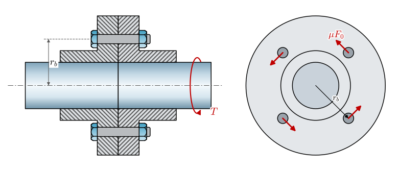
A rigid coupling makes the two shafts one. The simplest is a sleeve clamped over both shaft ends, a clamped hub with a hub on each side. The flange couplingsv. flänskoppling of Figure 9.14.3 puts a flange on each shaft end, keyed or shrunk on, and bolts the flanges face to face. The bolts are preloaded, the preload presses the faces together, and friction between the faces carries the torque, as in a bolted joint loaded in shear. With \(n_b\) bolts on the bolt circle of radius \(r_b\), each with the preload \(F_0\), and the friction coefficient \(\mu\) between the faces, the friction force at each bolt is \(\mu F_0\) and its moment arm \(r_b\), so the coupling carries before it slips
If it slips, the bolts take the torque in shear against the walls of their holes; the fitted bolts of heavy couplings are made for that. A friction coupling is designed not to slip, since slipping wears the faces and lets the preload go.
Figure 9.14.3: Example 1: a flange coupling. Left: in section, the flanges bolted face to face. Right: along the axis, four bolts on the bolt circle \(r_b\) and the friction force \(\mu F_0\) at each.
Example 1: A flange coupling
An electric motor of \(P = 15\) kW at \(n = 1460\) rpm drives a pump through the flange coupling of Figure 9.14.3: four M8 bolts of class 8.8 on a bolt circle of \(r_b = 40\) mm, preloaded to 70 % of their yield force as in Example 1 of the bolts chapter, with \(\mu = 0.15\) between dry steel faces. How large is the margin against slip?
The yield strength of class 8.8 is \(R_{p0.2} = 640\) MPa and the stress area of M8 is \(A_s = 36.6\) mm². The motor torque is \(T = P/\omega\).
Code
P_m, n_m =15e3, 1460# motor power [W] and speed [rpm]T_m = P_m/(2*np.pi*n_m/60) # motor torque [N m]F_0 =0.7*640*36.6# preload: 70 % of the yield force [N]n_b, r_b, mu_f =4, 0.040, 0.15T_slip = mu_f*n_b*F_0*r_b # torque at which the faces slip [N m]
The motor delivers far less than the faces can hold:
A margin of four looks generous, but the torque of a motor is not steady. An induction motor starting directly on the grid delivers two to three times its rated torque for a moment, and a pump that ingests air or a mill that jams adds shocks on top. The catalogues of coupling makers cover this with a service factor that multiplies the rated torque, and the margin here leaves room for a factor of two and a fair amount of preload lost to settling.
Flexible couplings
A flexible coupling lets the shafts be out of line, either by deforming or by sliding. The jaw couplingsv. klokoppling of Figure 9.14.1 has three jaws on each hub, and an elastomer spider with six arms sits between them. Each jaw pushes on an arm, so the arms carry the torque in compression, and because rubber or polyurethane is soft, the spider lets the hubs tilt by about a degree [1] and move sideways by a few tenths of a millimetre. It also damps the torque shocks of the motor and the load, and if the spider wears out, the jaws still drive each other metal on metal, so the drive keeps running, noisily, instead of coming apart. Bellows couplings and disc couplings use a thin metal part that bends instead: they take less misalignment than the jaw coupling but have no play at all and are stiff in torsion, as the drives of machine tools and 3D printers need.
The Oldham coupling
The Oldham couplingsv. Oldhamkoppling takes a parallel offset by sliding (Figure 9.14.4). Each hub has a slot across its face, and a disc between the hubs carries a tongue on each side, the two tongues at right angles. The input hub’s slot passes through the input axis and turns with it, so the disc can only slide along that slot, and the output’s slot, at right angles to it, passes through the output axis. The disc’s tongues are fixed to it at right angles, so the disc turns exactly as both hubs do: the coupling has a speed ratio of exactly one, whatever the offset.
Figure 9.14.4: An Oldham coupling with the output 7 mm above the input. The blue disc slides in both slots at once; its centre runs twice round a circle whose diameter is the offset, while the coupling turns once.
Where is the disc’s centre? It lies on the input slot, through the input axis \(O_1\), and on the output slot, through the output axis \(O_2\), and the two slots are at right angles. Seen from the centre, the two axes are at right angles, so by Thales’ theorem the centre lies on the circle with \(O_1O_2\) as its diameter. With the input turned by \(\theta\) from the line \(O_1O_2\), the centre is at the distance \(e\cos\theta\) from \(O_1\) along the input slot, and its position is
The centre runs round the circle of radius \(e/2\) at twice the shaft speed. The disc of mass \(m\) needs a centripetal force of \(m(e/2)(2\omega)^2\) from the slots,
\[
F_c = 2\,m\,e\,\omega^2
\tag{9.14.3}\]
which turns with the disc at twice the shaft speed and shakes the bearings. The disc also slides back and forth in each slot: its distance \(e\cos\theta\) from the input axis changes at the speed \(e\omega\sin\theta\), and the friction of that sliding wears the tongues and costs power. Both grow with the offset, and the Oldham coupling suits small offsets at moderate speed.
Example 2: An Oldham coupling at 1500 rpm
The Oldham coupling of Figure 9.14.4 connects a motor at \(n = 1500\) rpm to a pump. Its disc has a mass of \(m = 0.12\) kg. Find the rotating force on the bearings and the largest sliding speed, for the offset \(e = 0.5\) mm that the coupling is sold for and for the 7 mm of the animation.
Code
m_disc, n_o =0.12, 1500w_o =2*np.pi*n_o/60F_c = {e: 2*m_disc*e*w_o**2for e in (0.5e-3, 7e-3)} # @eq-cp-oldham-force [N]v_s = {e: e*w_o for e in (0.5e-3, 7e-3)} # largest sliding speed [m/s]
At the half millimetre it is designed for, the coupling shakes the bearings with 3 N, too little to notice. At 7 mm the force is fourteen times larger, and the tongues slide fourteen times as fast, at 1.1 m/s, under the full torque; the wear and the friction loss grow with them.
The Schmidt coupling
The Schmidt coupling takes large parallel offsets without sliding (Figure 9.14.5). It has three discs in a row: the outer two sit on the shafts and the middle one floats. Three links of equal length \(L\) join the input disc to the middle disc, and three more join the middle disc to the output disc; the pins sit on circles of equal radius, 120° apart. As the offset changes, the middle disc moves, but none of the discs turns relative to another.
Figure 9.14.5: A Schmidt coupling whose offset swings from \(0.5L\) to \(1.7L\) while it turns. The middle disc moves, and the red line painted on each disc stays parallel to the others: the output keeps the angle of the input.
The reason is the parallelogram. Two links of equal length between two discs whose pins sit on equal circles at the same angles form a parallelogram with the line between the pins on each disc, and a body held to another by a parallelogram can translate but not turn relative to it. The links therefore force the middle disc to keep the angle of the input disc, and the output disc to keep the angle of the middle disc: the output turns with the input. The middle disc’s centre lies at the distance \(L\) from both outer centres, which fixes it for any offset \(0 < e < 2L\). A Schmidt coupling transmits constant speed at any offset in that range, and the offset can change while it runs; the links pass the torque as tension and compression, without a sideways force on the shafts.
The Hooke joint
When the shafts meet at an angle, the classical coupling is the Hooke joint, also called the universal or cardan joint (Figure 9.14.6). Each shaft ends in a fork, and a cross with four arms joins them: one pair of arms turns in the input fork, the other pair in the output fork. The tractor’s power take-off shaft and the drive shaft of a rear-wheel-drive car end in such joints. The joint passes torque at angles of up to 30° or more, but its output does not turn at the speed of its input.
Figure 9.14.6: A Hooke joint at \(\beta = 30^\circ\), the input on the right turning at constant speed. The red stripes on the two shafts start in line and drift apart and back twice per turn: the output runs ahead and falls behind, between \(\cos\beta\) and \(1/\cos\beta\) of the input speed.
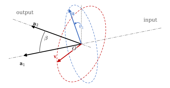
The kinematics follow from two conditions on the arms of the cross (Figure 9.14.7). Let the input axis be \(\bm{a}_1\) and the output axis \(\bm{a}_2\), at the angle \(\beta\), and measure the angles of both shafts from the plane that contains the two axes. The input fork holds the arm \(\bm{u}\), turning with the input in the plane normal to \(\bm{a}_1\); at the input angle \(\theta_1\),
in axes with \(\bm{a}_1\) along \(z\) and the plane of the shafts as the \(xz\) plane. The output fork holds the arm \(\bm{v}\), turning with the output in the plane normal to \(\bm{a}_2 = (\sin\beta, 0, \cos\beta)\). That plane is spanned by \(\bm{w} = (\cos\beta, 0, -\sin\beta)\), in the plane of the shafts, and \(\bm{e}_y\), normal to it, so at the output angle \(\theta_2\)
Figure 9.14.7: The Hooke joint as vectors: the input axis \(\bm{a}_1\), the output axis \(\bm{a}_2\) at the angle \(\beta\), the arm \(\bm{u}\) of the cross in the input fork, turned by \(\theta_1\) from the plane of the axes, and the arm \(\bm{v}\) in the output fork, at right angles to both \(\bm{u}\) and \(\bm{a}_2\). The dashed circles are the paths of the arm ends.
The two angles agree at every quarter turn, so on average the output keeps up, but in between it runs ahead and falls behind. Differentiating 9.14.4 with respect to time, \(\dot\theta_2/\cos^2\theta_2 = \dot\theta_1/(\cos^2\theta_1\cos\beta)\), and eliminating \(\theta_2\) with \(\cos^2\theta_2 = 1/(1 + \tan^2\theta_2)\) gives the speed ratio below; the cell checks it with SymPy.
Code
th1, beta = sp.symbols(r'theta_1 beta', real=True)ratio = sp.cos(beta)/(1- sp.sin(beta)**2*sp.cos(th1)**2) # @eq-cp-hooke-ratio# the ratio is the derivative of theta_2(theta_1) from @eq-cp-hooke-angletheta_2 = sp.atan(sp.tan(th1)/sp.cos(beta))assert sp.simplify(sp.diff(theta_2, th1) - ratio) ==0
The output speed is largest, \(\omega_1/\cos\beta\), when the input arm lies in the plane of the shafts (\(\theta_1 = 0\) and \(180^\circ\)), and smallest, \(\omega_1\cos\beta\), a quarter turn later. It swings between the two twice per revolution, as the graph in Figure 9.14.6 shows. The power passes through unchanged, apart from friction in the bearings of the cross, so the output torque swings the opposite way, \(T_2 = T_1\,\omega_1/\omega_2\). For small angles, \(\cos\beta \approx 1 - \beta^2/2\), and 9.14.5 becomes
The error grows with the square of the angle: about 1.5 % at 10°, 6 % at 20° and 14 % at 30°. Its rate of change matters as much as its size. A shaft that speeds up and slows down twice per turn has to be accelerated, and whatever inertia hangs on the output, a mower, a propeller, a wheel and the car behind it, has to be driven through that acceleration.
Example 3: The power take-off of a tractor
A tractor drives a rotary mower through a power take-off shaft with a Hooke joint at each end. The tractor’s shaft turns at the standard 540 rpm, and in a turn the first joint runs at \(\beta = 20^\circ\). Assume, for now, that the second joint is straight. The mower’s rotating parts have a moment of inertia of \(J = 0.5\) kg m² about their shaft. How much does the mower’s speed vary, and what torque does it take to accelerate the mower through the variation?
The output speed follows from 9.14.5. The output’s angular acceleration is \(\dot\omega_2 = \omega_1^2\, \mathrm{d}(\omega_2/\omega_1)/\mathrm{d}\theta_1\) at constant input speed, and the torque to drive it is \(J\dot\omega_2\).
Code
n_pto, beta_pto, J_mow =540, np.radians(20), 0.5w_pto =2*np.pi*n_pto/60n_out = (n_pto*np.cos(beta_pto), n_pto/np.cos(beta_pto)) # slowest and fastest [rpm]d_ratio = sp.lambdify((th1, beta), sp.diff(ratio, th1))th = np.linspace(0, np.pi, 20001)alpha_max = w_pto**2*np.max(np.abs(d_ratio(th, beta_pto))) # largest acceleration [rad/s^2]T_acc = J_mow*alpha_max # torque to drive it [N m]
The mower turns between the two speeds, with the largest acceleration and torque
The torque on the shaft swings by \(\pm 200\) N·m twice per revolution, 18 times per second, on top of the torque the mower needs to cut grass. That is a fatigue load on every part of the drive, and it is why the manuals for these shafts insist on two things: keep the angles small, and keep the two joints at equal angles with their forks in line. The next section shows why. The small-angle result, \(\dot\omega_{2,\max} \approx
\beta^2\omega_1^2\) from 9.14.6, gives 390 rad/s², within 3 % of the exact value.
Two Hooke joints
Two Hooke joints connected by an intermediate shaft can cancel each other’s error. The intermediate shaft has a fork at each end, and the question is how its second fork must sit relative to its first. Let the first joint turn the intermediate shaft by \(\theta_m\) with \(\tan\theta_m = \tan\theta_1/\cos\beta_1\), 9.14.4. If the intermediate shaft’s two forks lie in one plane, in line, and all three shafts lie in one plane, then at the second joint the intermediate shaft is the input and its arm starts a quarter turn from the plane of the shafts, where the first joint’s output arm \(\bm{v}\) started. The second joint obeys 9.14.4 with both angles shifted by a quarter turn, \(\tan(\theta_2 + \pi/2) = \tan(\theta_m + \pi/2)/\cos\beta_2\), and since \(\tan(x + \pi/2) = -\cot x\),
With equal angles, \(\beta_1 = \beta_2\), the output follows the input exactly: the second joint undoes what the first did. The intermediate shaft still speeds up and slows down, but it is light, and the shafts at both ends turn evenly. The input and output may be parallel, the intermediate shaft tilted between them (a Z layout), or meet at an angle with the intermediate shaft crossing between them (a W layout); in both the angles must be equal. Figure 9.14.8 shows what happens when the forks are not in line. Turned a quarter turn apart, the second joint adds its error to the first instead of cancelling it, and the output swings between \(\cos^2\beta\) and \(1/\cos^2\beta\) of the input speed.
Figure 9.14.8: Two Hooke joints at \(30^\circ\) each in a Z layout. Above, the forks of the intermediate shaft are in line and the output turns with the input. Below, the second fork is turned a quarter turn, and the errors add.
A double cardan joint puts the two joints close together in one housing, with a centring device that keeps the two angles equal, and is a compact constant-velocity joint.
Constant-velocity joints
The front wheels of a car are driven and steered, so their drive shafts need joints that run at large angles, change their angle all the time, and turn the wheel evenly. A single Hooke joint fails the last condition, and a pair cannot keep its two angles equal when the wheel steers. The ball joint that solves this, the Rzeppa joint and its descendants, sits at the outer end of the drive shafts of front-wheel-drive cars (Figure 9.14.9).
Figure 9.14.9: A ball joint at \(30^\circ\), the bell on the input shaft cut open. Six balls (red) run in grooves of the bell and of the inner race on the output shaft, and a cage (dark) holds them in the plane that bisects the angle between the shafts. The stripes on the shafts stay in line: input and output turn at the same speed.
The principle fits in two sentences. A ball touches both the bell and the inner race and drives one with the other at its contact points, so the point where it sits has the same velocity as a point of the input and as a point of the output. If that point lies in the plane that bisects the angle between the shafts, it is equally far, \(r\), from both axes, so \(\omega_1 r = \omega_2 r\) and the two shafts turn at the same speed. The grooves of the bell and the inner race are curved so that their crossing, and with it each ball, is pushed into that plane, and the cage keeps the balls there. The joint is homokineticsv. homokinetisk, a constant-velocity jointsv. drivknut or CV joint. The same argument shows why two Hooke joints with equal angles work: the arrangement is symmetric about the plane that bisects it.
The inner end of a car’s drive shaft usually has a tripod joint: three rollers on a spider, running in three straight grooves of a housing. It takes smaller angles but lets the shaft slide in and out; the outer ball joint cannot. As the suspension moves, the distance between the gearbox and the wheel changes, and the drive shaft has to change its length with it, by sliding in a tripod joint or in a spline (9.14.8).
The drive shafts of the RC car
The drive shafts of a hobby RC car face the same problem at a smaller scale, and the hobby’s names for the solutions are worth knowing. A dogbone is a short shaft with a ball at each end and a pin through each ball; the balls sit in cups with two slots that the pin ends run in. Each end lets the shaft tilt about the pin and about the axis across the slots, two axes at right angles through the ball centre, as in a Hooke joint, and the pin slides in the slots to take the change of length. A dogbone is a pair of Hooke joints with a plunge built in, and with the two pins parallel its forks are in line. A universal joins the shaft and the wheel axle with a pivot instead of a loose cup, and joints sold as CVD use a ball and pin arrangement meant to keep the wheel speed constant at any angle. Which of these the car of the course uses at the rear and at the front is the subject of the next example.
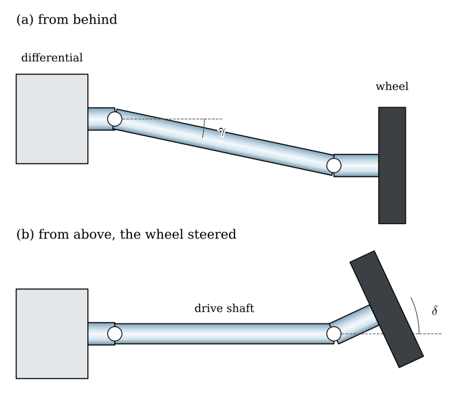
Figure 9.14.10: Example 4: the front drive shaft of the RC car. (a) From behind: the shaft falls by \(\gamma\) from the differential to the wheel, and the two outputs are level. (b) From above: the wheel steered by \(\delta\) about its kingpin, which passes through the outer joint.
Example 4: Dogbones on the front axle
The front drive shafts of the RC car of Figure 9.14.10 fall by \(\gamma = 12^\circ\) from the differential to the wheel, and each has a dogbone joint at each end with the two pins parallel. How evenly does the wheel turn when the car drives straight, and when the wheel is steered by \(\delta = 25^\circ\)?
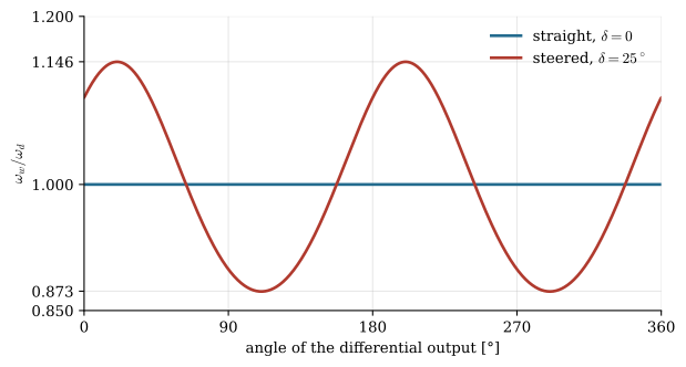
Driving straight, the differential output and the wheel axle are parallel and both joints run at \(12^\circ\): a Z layout with equal angles and forks in line, so by 9.14.7 the wheel turns evenly. Steered, the wheel axle turns by \(\delta\) about the vertical kingpin through the outer joint, and the angle at the outer joint grows, while the inner one stays at \(\gamma\). The angle between the shaft and the steered axle follows from the dot product of their directions; the speed ratio over a turn follows from the two-joint construction of 9.14.7, carried out with vectors by the script tools/blender/coupling_system.py, the same functions that drive the animations.
Code
sys.path.insert(0, '../tools/blender')import coupling_system as csgam, dlt = np.radians(12), np.radians(25)a_diff = np.array([0, 1.0, 0]) # differential output, across the cara_shaft = np.array([0, np.cos(gam), -np.sin(gam)]) # the drive shaft, falling by gammaa_wheel = np.array([-np.sin(dlt), np.cos(dlt), 0]) # the wheel axle, steered by deltabeta_2 = np.arccos(a_shaft @ a_wheel) # angle at the outer jointth = np.linspace(0, 2*np.pi, 2001)ref = cs.unit(np.cross(a_wheel, np.cross([0, 0, 1.0], a_wheel)))def wheel_speed(a_out, ref_out):"""omega_wheel/omega_diff over one turn, forks of the dogbone in line.""" ang = [cs.angle_about(cs.double_cardan(t, a_diff, a_shaft, a_out)[3], a_out, ref_out) for t in th]return np.gradient(np.unwrap(ang), th)w_straight = wheel_speed(np.array([0, 1.0, 0]), np.array([0, 0, 1.0]))w_steered = wheel_speed(a_wheel, ref)
Figure 9.14.11: The wheel speed over one turn of the differential output in Example 4, driving straight and with the wheel steered by 25°, both with dogbone joints with parallel pins.
Straight, the wheel turns evenly, as 9.14.7 promises. Steered by 25°, the outer joint runs at 27.6° against 12° at the inner one, the cancellation fails, and the wheel speeds up and slows down by about 14 % twice per turn of the shaft (Figure 9.14.11). At full throttle in a turn, that is a torque pulsation at the front wheels that the driver feels as a judder in the steering and that hammers the joints. The rear wheels of the car do not steer, so dogbones serve there; the front wheels need joints that stay homokinetic at the outer end, a ball joint or a joint sold as CVD, and that is where they are worth their price.
Splines
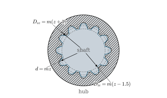
A coupling, a gear or a wheel hub has to take the torque off the shaft, and the shaft–hub joints chapter treats the key, the pin and the press fit. The spline is the shape-locked joint for large torques and for hubs that must slide: the gearbox shafts on which the gears are shifted, the yokes that slide on a power take-off shaft as the tractor turns, the inner end of a car’s drive shaft, and the cassette of a bicycle. Its teeth are the teeth of a gear with a short addendum. ISO 4156[2] specifies involute splines with pressure angles of 30°, 37.5° and 45°; at 30° with a flat root, the shaft of \(z\) teeth and module \(m\) has the pitch diameter \(d = mz\), like a gear, the major diameter \(D_{ee} = m(z + 1)\) and the minor diameter \(D_{ie} = m(z - 1.5)\), and the hub’s teeth reach down to about \(m(z - 1)\) (Figure 9.14.12). The flanks overlap over the radial depth \(h = (D_{ee} - m(z - 1))/2 = m\).
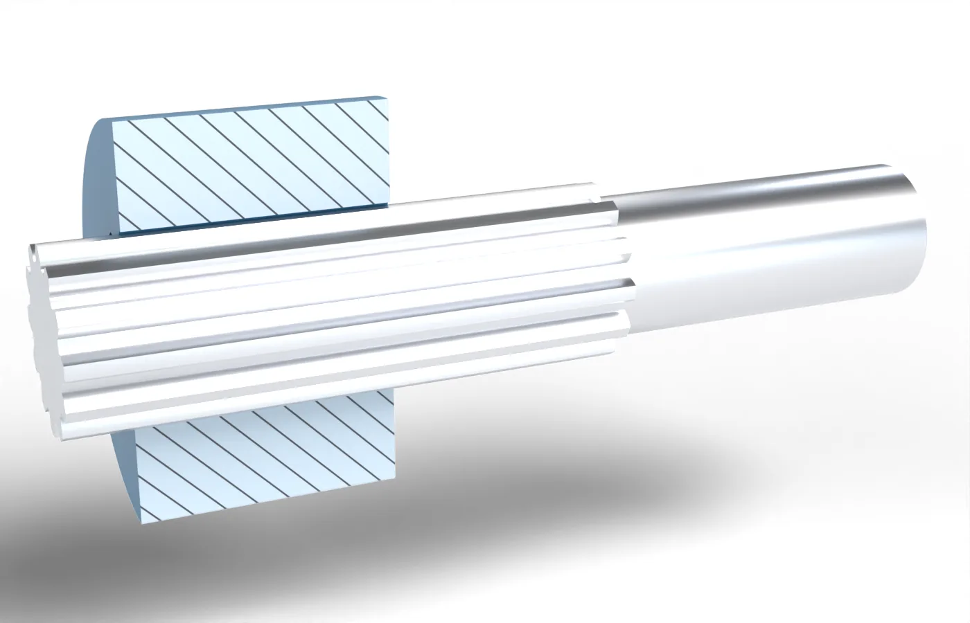
Figure 9.14.12: An involute spline of ISO 4156 with 12 teeth of module 1.5 at 30°. Above, the section, the shaft in its hub. Below, the hub cut open lengthwise on the shaft, the teeth running out beyond it.
The involute flanks centre the hub on the shaft under load, as the teeth of a gear centre each other, and the hub can be pushed along the teeth while it carries torque. The torque \(T\) reaches each tooth as a force at the pitch radius \(d/2\), and like the parallel key the teeth are checked against the bearing pressure on the projected flank \(h L\) over the hub length \(L\). The teeth are never cut exactly alike, so not all of them carry; as the shaft–hub chapter notes, the design rules count about three quarters of them, \(\varphi = 0.75\). The bearing pressure is then
\[
p = \frac{2T}{d\,\varphi\, z\, h\, L}
\tag{9.14.8}\]
Example 5: Spline or key?
A hub \(L = 25\) mm long carries \(T = 150\) N·m on the spline of Figure 9.14.12, 12 teeth of module 1.5. Compare its bearing pressure with that of a parallel key 6 × 6 on a plain shaft of the same pitch diameter, 18 mm, with the depth \(t_1 = 3.5\) mm in the shaft, so that \(h - t_1 = 2.5\) mm of the key bears on the hub.
Code
T_s, L_s, z_s, m_s, phi_s =150.0, 25.0, 12, 1.5, 0.75d_s = m_s*z_s # pitch diameter [mm]p_spline =2*T_s*1e3/(d_s*phi_s*z_s*m_s*L_s) # @eq-cp-spline, h = m [MPa]p_key = (2*T_s*1e3/d_s)/(2.5*L_s) # key: F = 2T/d on (h - t1) L [MPa]
The key bears on 2.5 mm of one face, the spline on 1.5 mm of nine; the spline carries the torque at a fifth of the pressure, about 50 MPa, and a hub of ordinary steel takes that with a large margin, while the 270 MPa on the key face is beyond what a hub of structural steel can bear (the yield strength of S355 is 355 MPa, and a factor of safety leaves well under 200). The spline also leaves the shaft round on average: it weakens it less than a keyway and does not set up the stress concentration at the end of a key seat.
A related shape lock is the polygon of the shaft–hub chapter: a shaft of rounded triangular or square section with no teeth at all. It carries torque by wedging, centres the hub as it does so and has no notches; the toolholders of machine tools (Coromant Capto) and some motor shafts use it.
Printed couplings
Most couplings in the RC car are printed, and printing changes what works. A printed hole is never round to better than a tenth of a millimetre, so a printed hub on a round motor shaft slips unless something locks it: a flat on the shaft with a matching D-shaped bore, a set screw in a nut trap, or a hexagon. The wheel hubs of hobby cars sit on a 12 mm hexagon, a polygon in the sense of 9.14.8, and the hexagon prints well because its flat faces are made from straight lines in every layer. Jaw couplings print well too, with a spider printed in TPU, and they forgive the misalignment between a motor and a printed gearbox that a rigid printed coupling would turn into cracks.
What printing does not give is strength in the pins and balls of a joint. A dogbone pin loads the ball across the layers, the weakest direction of a printed part, and the pins of the car’s joints are steel, pressed into printed or bought balls. How much torque a printed jaw coupling or a printed hexagon hub carries, and how the layer direction changes it, has to be measured; we will test them on the universal testing machine and report the results here.
TipIn industry: choosing from the catalogue
Couplings are bought, not designed. A catalogue lists for each size the nominal torque \(T_{KN}\), the largest permitted offset, angle and axial movement, and the largest speed. The designer multiplies the torque of the drive by a service factor\(K_A\) for the kind of machine, close to 1 for an electric motor driving a fan and 2 or more for a piston engine driving a crusher, and chooses the smallest coupling with \(T_{KN} \ge K_A T\). The permitted misalignments are for the coupling’s life, so they are checked against what the installation will actually have, and the shafts are aligned with a laser alignment tool when the machine is installed; most coupling failures are decided there. Cardan shafts and drive shafts with ball joints are bought the same way, with the joint angle and the length change of the installation as the inputs.
Problems
Problem 1: Six bolts. The flange coupling of Example 1 gets six M8 bolts instead of four, on the same circle. A service factor of \(K_A = 2\) applies. What margin against slip remains, and how many bolts would \(K_A = 3\) need for a margin of 1.5?
Answer:Six bolts carry 590 N·m against \(2 \cdot 98 = 196\) N·m, a margin of 3.0. With \(K_A = 3\) the torque is 294 N·m, and a margin of 1.5 asks for 441 N·m, so \(441/98.3 = 4.5\), five bolts, in practice six for symmetry.
Problem 2: How large an angle? A Hooke joint drives a machine whose speed may vary by at most ±2 %. What is the largest joint angle?
Answer:With 9.14.6 the speed swings by \(\pm\beta^2/2\) about the mean, so \(\beta^2/2 \le 0.02\) gives \(\beta \le 0.2\) rad, about 11°. The exact 9.14.5 gives \(1/\cos\beta \le 1.02\), \(\beta \le 11.4^\circ\).
Problem 3: The PTO with both joints. The tractor of Example 3 has its second joint at 20° too, and the forks of the intermediate shaft in line. What does the mower see? What if the user, after taking the shaft apart, puts the two halves back a quarter turn apart?
Answer:In line and at equal angles the second joint cancels the first, 9.14.7, and the mower turns evenly. A quarter turn apart, the errors add: the speed swings between \(\cos^2 20^\circ = 0.88\) and \(1/\cos^2 20^\circ = 1.13\) of 540 rpm, twice the variation of one joint, and the torque to accelerate the mower roughly doubles to about 400 N·m.
Problem 4: A Schmidt coupling. The links of a Schmidt coupling are 60 mm long. Over what range of offsets does it work, and where is the middle disc’s centre at the offset \(e = 80\) mm?
Answer:For \(0 < e < 2L = 120\) mm. The centre is at the distance \(L\) from both outer centres: halfway along, \(e/2 = 40\) mm, and \(\sqrt{L^2 - (e/2)^2} = 44.7\) mm to the side of the line between them.
Problem 5: A spline for the RC car. A printed hub 10 mm long must carry 1.5 N·m, an assumed torque at one rear wheel of the RC car, on a steel spline of 10 teeth and module 0.5. What bearing pressure does it see, and is that acceptable for PLA, whose compressive yield strength we take as 60 MPa?
Answer:\(d = 5\) mm, \(h = 0.5\) mm, and 9.14.8 gives \(p = 2 \cdot 1500/(5 \cdot 0.75 \cdot 10 \cdot 0.5 \cdot 10) = 16\) MPa, a factor of 3.75 to 60 MPa. Acceptable as a static check, but teeth of 0.5 mm module are about one extrusion width deep and will not print accurately; a hexagon would serve better.
Further reading
Budynas and Nisbett [1] show the common shaft couplings as they appear in catalogues and treat the positive and overrunning clutches that are related to them. ISO 4156 [2] gives the geometry and tolerances of involute splines. The coupling makers’ catalogues are the practical reference for ratings, service factors and permitted misalignments, and the shaft–hub joints chapter covers the keys, pins and fits that hold a coupling’s hub on its shaft. Brakes and clutches, which couple and uncouple shafts while they run, are the subject of their own chapter.