9.7 Cycloidal and strain wave drives
A robot joint needs a ratio of 30 to 160 between a fast motor and a slow arm, with little backlash, in a flat housing on the joint’s axis. A planetary gear reaches 3 to 10 in one stage, so it needs two or three. The two drives of this chapter reach the whole range in one stage, by letting a part wobble or bend inside a ring that has one or two teeth more. In the cycloidal drivesv. cykloidväxel a disc with lobes rolls around a ring of pins on an eccentric; in the strain wave gearsv. harmonisk växel, sold as the Harmonic Drive, a thin toothed cup is bent into an ellipse and rolls inside a rigid ring. Both are planetary gears in disguise: the eccentric and the bent shape are carriers, and the Willis equation gives their ratios.
The chapter derives the shape of the cycloid disc from a rolling circle, shows why every pin touches it, and finds the conditions under which the disc can be made. It then explains the strain wave gear and the stress that limits it, the bending of the flexspline, and closes with what tests of 3D-printed drives show about the three kinds.
The cycloidal drive
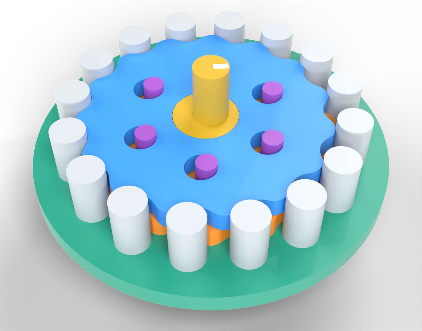
Figure 9.7.1 shows a cycloidal drive. The input shaft (yellow) carries an eccentric, a crank of radius \(e\), and a disc with \(n - 1\) lobes turns freely on it. Around the disc stands a ring of \(n\) pins fixed in the housing (teal and grey). The eccentric pushes the disc around the inside of the pin ring, and since the disc has one lobe fewer than there are pins, it cannot follow the eccentric round: each lobe rolls into the next gap between the pins, and after a full turn of the eccentric the disc has turned back by one lobe, \(1/(n-1)\) of a turn. Six pins of an output flange (purple) reach through holes in the disc and pick up its slow rotation. Two discs half a turn apart (orange and blue) balance each other.
The drive was patented by Lorenz Braren; according to [1], the number of rollers differs by one from the number of teeth of the disc, whose profile is an epitrochoid, and the crank and the slow shaft turn in opposite directions.
The ratio
The eccentric is the carrier. Seen from it, the disc and the pin ring are an internal gear pair of \(n - 1\) and \(n\) teeth, which turn in the same sense, so 9.6.2 becomes, with the disc in the place of the sun,
\[ \frac{\omega_d - \omega_e}{\omega_\text{pins} - \omega_e} = \frac{n}{n - 1} \]
With the pins in the housing, \(\omega_\text{pins} = 0\), and the disc turns at
\[ \omega_d = \omega_e\left(1 - \frac{n}{n - 1}\right) = -\frac{\omega_e}{n - 1}, \qquad i = -(n - 1) \tag{9.7.1}\]
backwards, \(n - 1\) times slower than the input. The drive of Figure 9.7.1 has \(i = -15\); in a test of two printed drives, 26 pins gave \(-25\) [2]. The same ratio is given by [3] for one stage, \(u = z_1/(z_2 - z_1)\) with \(z_1\) lobes and \(z_2\) rollers.
The disc profile: a rolling circle
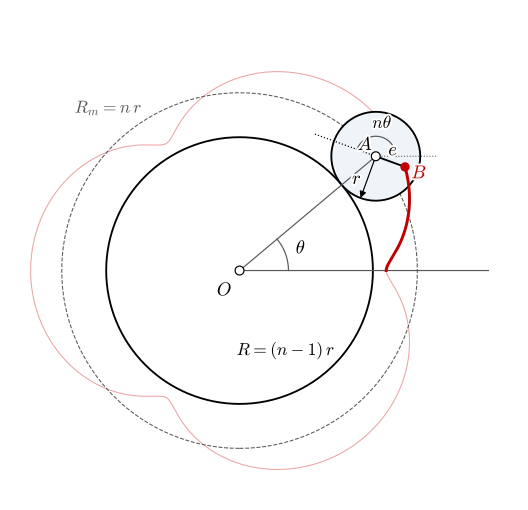
The disc must touch every pin at every instant. Its shape comes from a rolling circle (Figure 9.7.2). A circle of radius \(r\) rolls without slipping around the outside of a fixed base circle of radius \(R = (n - 1)\,r\). Its centre \(A\) runs on the circle of radius \(R + r = nr\), which is the pin circle \(R_m\):
\[ r = \frac{R_m}{n},\qquad R = (n - 1)\,r,\qquad \bm r_A = R_m\begin{bmatrix}\cos\theta\\ \sin\theta\end{bmatrix} \]
When \(A\) has moved by \(\theta\), the arc \(R\theta\) of the base circle has rolled off on the arc \(r\varphi\) of the rolling circle, so the rolling circle has turned by \(\varphi = (R/r)\,\theta = (n-1)\,\theta\) relative to the line \(OA\). The line \(OA\) has itself turned by \(\theta\), so against the fixed frame the rolling circle has turned by
\[ \theta + \varphi = n\,\theta \]
one turn more per orbit than the arcs suggest. This extra turn is the coin rotation paradox: a coin rolled around an equal coin turns twice, not once [4]. Using \((n-1)\theta\) as the angle of the tracing arm is an easy slip, and it gives a curve with \(n - 2\) lobes instead of \(n - 1\).
A point \(B\) fixed to the rolling circle at the distance \(e\) from its centre, which starts on the line \(OA\) towards \(O\), then traces
\[ \bm r_B(\theta) = R_m\begin{bmatrix}\cos\theta\\ \sin\theta\end{bmatrix} - e\begin{bmatrix}\cos n\theta\\ \sin n\theta\end{bmatrix} \tag{9.7.2}\]
an epitrochoid [5] with \(n - 1\) lobes. With \(e = r\) the point lies on the rolling circle and the curve is an epicycloid with sharp cusps; with \(e < r\) it is smooth. The ratio
\[ K_1 = \frac{e\,n}{R_m} = \frac{e}{r} \tag{9.7.3}\]
is called the short width coefficient [6], which recommends \(K_1\) between 0.48 and 0.74 for discs of 13 to 23 lobes and between 0.65 and 0.9 for 25 to 59.
Why every pin touches the disc
The curve of 9.7.2 is the path of a pin centre seen from the disc. Let the eccentric stand at the angle \(\psi\), so the disc centre is at \(e[\cos\psi,\ \sin\psi]\), and let the disc have turned by \(-\psi/(n-1)\) as 9.7.1 says. Pin \(k\) stands at \(R_m[\cos\alpha_k,\ \sin\alpha_k]\) with \(\alpha_k = 2\pi k/n\). In the disc’s own frame, turned back by \(\psi/(n-1)\), the pin centre is at
\[ \bm{\mathsf R}\!\left(\tfrac{\psi}{n-1}\right) \left(R_m\begin{bmatrix}\cos\alpha_k\\ \sin\alpha_k\end{bmatrix} - e\begin{bmatrix}\cos\psi\\ \sin\psi\end{bmatrix}\right) = R_m\begin{bmatrix}\cos\theta_k\\ \sin\theta_k\end{bmatrix} - e\begin{bmatrix}\cos\frac{n\psi}{n-1}\\ \sin\frac{n\psi}{n-1}\end{bmatrix} \]
with \(\theta_k = \alpha_k + \psi/(n-1)\) and \(\bm{\mathsf R}\) the rotation matrix. Since \(n\theta_k = 2\pi k + n\psi/(n-1)\), the last vector is \(e[\cos n\theta_k,\ \sin n\theta_k]\), and the pin centre lies on \(\bm r_B(\theta_k)\): every pin centre stays on the curve, at every input angle. The disc is the curve moved inwards by the pin radius \(r_p\) along its normal,
\[ \bm r_\text{disc} = \bm r_B - r_p\,\bm n,\qquad \bm n = \frac{1}{|\bm r_B'|}\begin{bmatrix}y_B'\\ -x_B'\end{bmatrix} \tag{9.7.4}\]
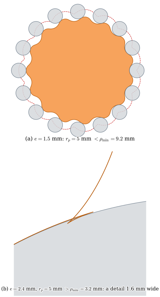
with \(\bm n\) the outward unit normal, so every pin of radius \(r_p\) touches the disc. The moved curve is free of loops only while \(r_p\) is smaller than the curve’s smallest radius of curvature \(\rho_\text{min}\) where it is convex, on the shoulders of each valley; a larger pin cuts the disc there (Figure 9.7.3).
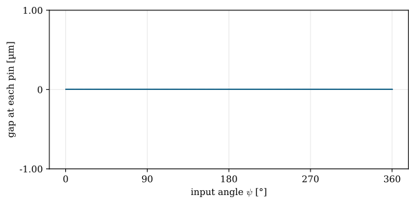
The check is easily made numerically: for any input angle, place the pins, move them into the disc’s frame, and measure the distance from each pin centre to the disc outline, which should be \(r_p\). Figure 9.7.4 plots the gap, the distance minus \(r_p\), for all 16 pins of Figure 9.7.1 over one turn of the input.
Code
n, R_m, e, r_p = 16, 40.0, 1.5, 5.0
x, y = cycloid_disc(n, R_m, e, r_p, n=20000)               # @eq-cs-offset, disc frame
disc = np.c_[x, y]
alpha = 2*np.pi*np.arange(n)/n
psis = np.linspace(0, 2*np.pi, 73)
gap = np.empty((len(psis), n))
for i, psi in enumerate(psis):
    c, s = np.cos(psi/(n - 1)), np.sin(psi/(n - 1))          # the disc turned back by psi/(n-1)
    pins = R_m*np.c_[np.cos(alpha), np.sin(alpha)] - e*np.array([np.cos(psi), np.sin(psi)])
    pins = pins @ np.array([[c, s], [-s, c]])                # into the disc's frame
    d = np.linalg.norm(disc[None, :, :] - pins[:, None, :], axis=2).min(axis=1)
    gap[i] = d - r_p
fig, ax = plt.subplots(figsize=(6.4, 3.2))
ax.plot(np.degrees(psis), gap*1e3, color='#236B8E', lw=0.8)
ax.set_xlabel(r'input angle $\psi$ [°]')
ax.set_ylabel(r'gap at each pin [µm]')
ax.set_xticks([0, 90, 180, 270, 360])
lim = max(1.0, np.abs(gap).max()*1e3*1.2)
ax.set_ylim(-lim, lim)
ax.set_yticks([-lim, 0, lim])
ax.set_yticklabels([f'{-lim:.2f}', '0', f'{lim:.2f}'])
ax.grid(alpha=0.3)
plt.tight_layout()
plt.show()The largest gap is a fraction of a micrometre, the resolution of the 20 000 points of the outline: in theory every pin touches the disc. Half of them carry load, the ones on the side the eccentric pushes towards; the others touch without force.
Example 1: a disc for a robot joint
A cycloidal drive for a robot joint has \(n = 21\) pins of radius \(r_p = 10\) mm on a pin circle of radius \(R_m = 81.27\) mm (Figure 9.7.5). Find the ratio, and check whether a disc can be made with the eccentricity equal to the rolling circle radius, \(e = r\), and with \(e = 3.0\) and \(2.5\) mm.
9.7.1 gives \(i = -(n-1)\), 9.7.3 gives \(K_1\), and the disc can be made if \(r_p < \rho_\text{min}\).
Code
n1, Rm1, rp1 = 21, 81.27, 10.0
r1 = Rm1/n1
ex1 = {lab: (ee, ee*n1/Rm1, cycloid_min_radius(n1, Rm1, ee)) for lab, ee in
       (('e = r', r1), ('e = 3.0', 3.0), ('e = 2.5', 2.5))}
The rolling circle has \(r = R_m/n\); for the three eccentricities, \(K_1\) and the smallest radius of curvature are
\[ \begin{aligned}r &=3.87~\text{mm},\quad i = -20\\e = r:\quad K_1 &=1.0,\quad \rho_\text{min} =0~\text{mm}\\e = 3.0:\quad K_1 &=0.775,\quad \rho_\text{min} =11.6~\text{mm}\\e = 2.5:\quad K_1 &=0.646,\quad \rho_\text{min} =14.0~\text{mm}\end{aligned} \]
With \(e = r\) the curve is the epicycloid with cusps, \(\rho_\text{min} = 0\), and no pin of finite radius fits; a CAD program that offsets the curve anyway trims the loops and leaves a disc that touches the pins only in part of the turn. With \(e = 3.0\) mm the disc can be made, \(\rho_\text{min} = 11.6\) mm \(> 10\) mm, but \(K_1 = 0.78\) lies above the 0.74 that [6] recommends for 20 lobes, and the margin to the pin radius is small. With \(e = 2.5\) mm, \(K_1 = 0.65\) is inside the range and \(\rho_\text{min} = 14\) mm leaves room. A smaller \(e\) makes the lobes shallower, and the contact force on each pin steeper to the direction of motion, so \(K_1\) is a compromise between a disc that can be made and one that pushes the pins efficiently.
The output: pins in holes
The disc wobbles on a circle of radius \(e\) while it turns slowly, and the output shaft must take the slow turning without the wobble. That is a parallel offset of \(e\), the job of the Oldham and Schmidt couplings: here a ring of \(k\) output pins of radius \(r_o\) on the output flange reaches through holes of radius \(r_o + e\) in the disc. The hole centres move on circles of radius \(e\) around the pin centres, so each pin rolls around the inside of its hole and touches it at every instant, and the flange turns exactly with the disc.
A single disc is unbalanced: its centre runs round at the input speed on the radius \(e\), as the disc of an Oldham coupling does, and needs the force \(m_d e\omega^2\). Two discs on two eccentrics half a turn apart cancel the force, though their two forces, a disc thickness apart, still form a rotating couple. The second disc is the first turned half a turn about its own centre, and it seats on the pins only if the number of lobes is odd [7]. In the disc’s frame it must sit like the first disc does after the input has turned half a turn, which by 9.7.1 has turned the disc by \(-\pi/(n-1)\); turning a disc of \(n - 1\) lobes by \(\pi\) instead gives the same picture only if \(\pi\) and \(-\pi/(n-1)\) differ by a whole number of lobes, \(2\pi/(n-1)\). That holds when \(n - 1\) is odd. Figure 9.7.6 shows both cases.
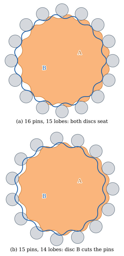
Example 2: the odd number of lobes
Check the rule of Figure 9.7.6 numerically: for 15 and 16 pins, find the smallest clearance between the second disc and the pins at the input angle zero.
The second disc has its centre at \(-e\) and is the outline of 9.7.4 turned by \(\pi\). The clearance of a pin is the distance from its centre to the outline minus \(r_p\), negative where the disc cuts the pin.
Code
clear = {}
for n2 in (15, 16):
    x2, y2 = cycloid_disc(n2, R_m, e, r_p, n=20000)
    disc_b = np.c_[-x2, -y2] + np.array([-e, 0])              # turned by pi, centre at -e
    pins = R_m*np.c_[np.cos(2*np.pi*np.arange(n2)/n2), np.sin(2*np.pi*np.arange(n2)/n2)]
    d = np.linalg.norm(disc_b[None, :, :] - pins[:, None, :], axis=2).min(axis=1)
    inside = Path(disc_b).contains_points(pins)               # a pin centre inside the disc
    clear[n2] = np.round(np.where(inside, -d - r_p, d - r_p).min(), 6) + 0.0
The smallest clearance in mm, for 15 pins (14 lobes) and 16 pins (15 lobes):
\[ \begin{aligned}n = 15:\quad c_\text{min} &=-2.96~\text{mm}\\ n = 16:\quad c_\text{min} &=0~\text{mm}\end{aligned} \]
With 16 pins the second disc touches every pin, a clearance of zero, and with 15 pins it cuts 3 mm into some of them: the 14-lobe drive of the test in [7] could not be assembled with two discs, and was rebuilt with 15 lobes and 16 pins.
The strain wave gear
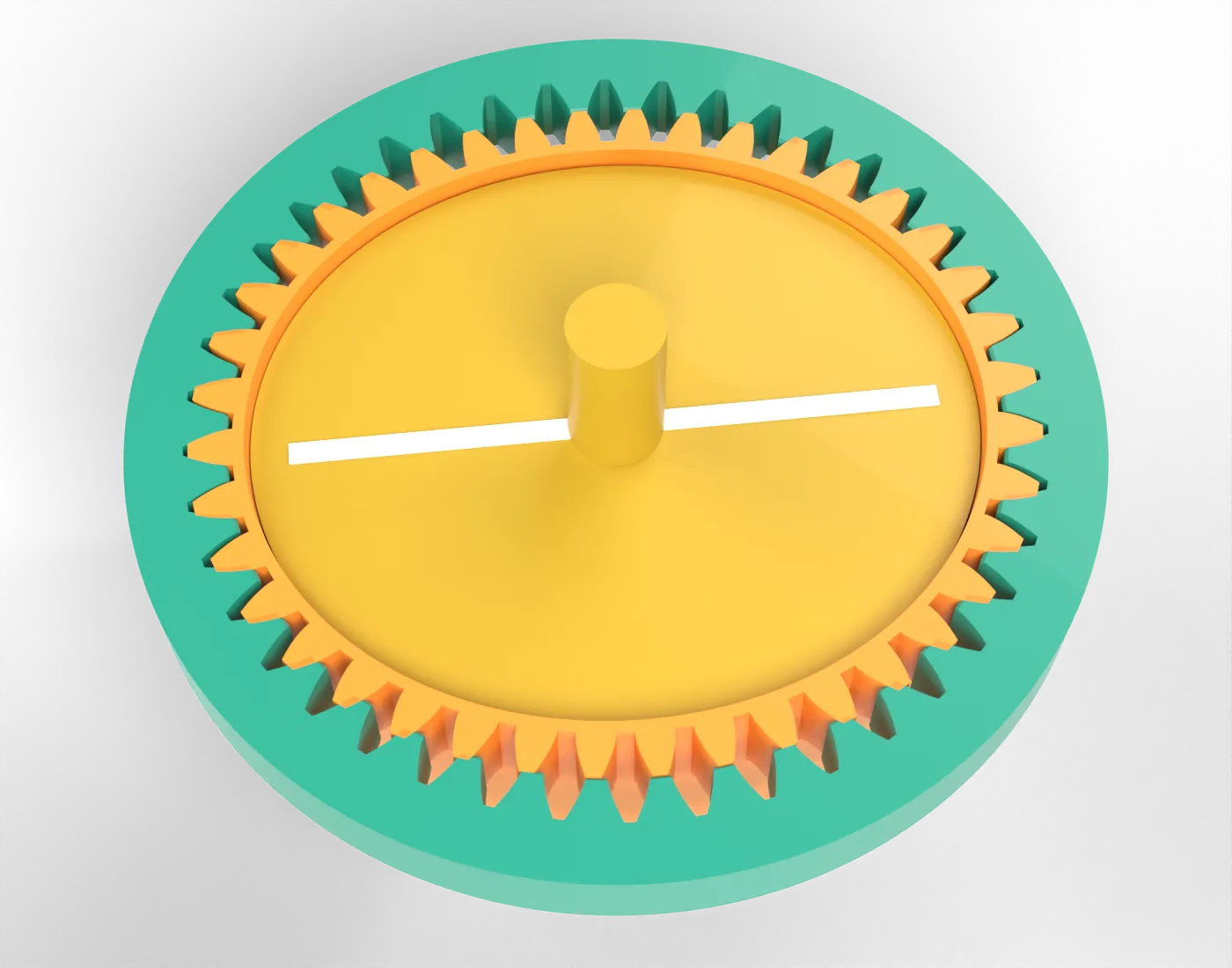
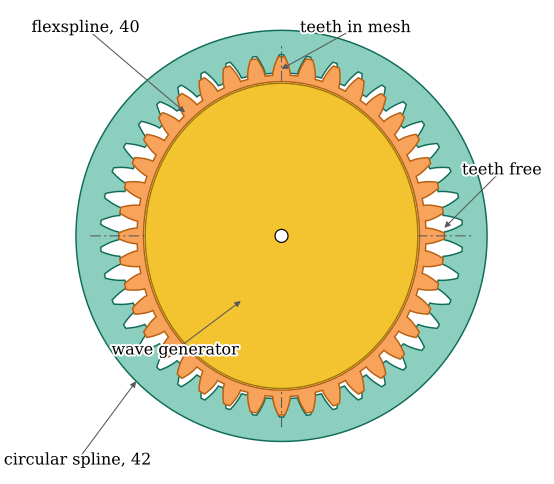
The strain wave gear has three parts (Figure 9.7.7). The circular splinesv. cirkulär spline is a rigid ring with \(N_c\) internal teeth, fixed in the housing. Inside it sits the flexsplinesv. flexspline, a thin-walled steel cup with \(N_f = N_c - 2\) external teeth around its open end; its bottom is the output flange. The wave generatorsv. vågenerator, an elliptical cam with a thin ball bearing on it, turns inside the flexspline and bends it into an ellipse. At the two ends of the major axis the teeth of the flexspline mesh fully with the circular spline; across the minor axis they are free. The invention is Musser’s [8], whose patent asks for a tooth difference equal to the number of points where the cup is pushed out, two for an elliptical cam.
The ratio
As the wave generator turns, the two zones of mesh travel round with it. Each half turn moves the mesh across one tooth of the circular spline, and since the flexspline has two teeth fewer it falls behind: after a full turn of the wave generator it has turned back by two teeth [9]. The wave generator is the carrier, and seen from it the flexspline and the circular spline are an internal pair of \(N_f\) and \(N_c\) teeth:
\[ \frac{\omega_f - \omega_w}{\omega_c - \omega_w} = \frac{N_c}{N_f} \]
With the circular spline fixed,
\[ \omega_f = \omega_w\left(1 - \frac{N_c}{N_f}\right) = -\frac{N_c - N_f}{N_f}\,\omega_w, \qquad i = -\frac{N_f}{N_c - N_f} = -\frac{N_f}{2} \tag{9.7.5}\]
the ratio is half the number of teeth of the flexspline, and the output turns backwards [10]. Musser’s example has 200 and 198 teeth for 100:1, and standard ratios run from 30 to 160 [11]. The many teeth in mesh at once, about a third of them at each end of the major axis, and the preload of the bent cup give the strain wave gear its zero backlash.
The bending of the flexspline
The pitch diameters of the two splines differ by \(m(N_c - N_f) = 2m\). To mesh at the ends of the major axis, the flexspline must be pushed out there by half of that, the radial deflection
\[ w_0 = \frac{m\,(N_c - N_f)}{2} = m \]
which is why the tooth difference is kept at two: a larger difference needs a larger deflection. The wave generator bends the wall of radius \(R\) into the shape \(w(\phi) = w_0\cos 2\phi\). A thin ring that is bent without being stretched changes its curvature by \(\Delta\kappa = -(w + w'')/R^2\), the second derivative taken with respect to \(\phi\), and with \(w'' = -4w\),
\[ \Delta\kappa = \frac{3\,w_0}{R^2}\cos 2\phi \]
The wall of thickness \(t\) bends with the strain \(\varepsilon = \Delta\kappa\, t/2\) at its surfaces, so the largest bending strain and stress are
\[ \varepsilon_\text{max} = \frac{3\,t\,w_0}{2R^2},\qquad \sigma_\text{max} = E\,\varepsilon_\text{max} \tag{9.7.6}\]
and they change sign twice per turn of the wave generator, as the ellipse passes. Every point of the cup therefore sees two full stress cycles for each input turn, a fatigue load: at 3000 rpm, \(10^7\) cycles take about a day. The flexspline is made thin to keep \(\varepsilon\) small, and its life, with that of the wave generator’s bearing, is what limits a strain wave gear.
The curvature change is easily checked numerically: the curve \(\rho(\phi) = R + w(\phi)\) in polar form has the curvature \(\kappa = (\rho^2 + 2\rho'^2 - \rho\rho'')/(\rho^2 + \rho'^2)^{3/2}\), and Figure 9.7.8 compares it with \(1/R + \Delta\kappa\).
Code
R_f, w_0 = 35.0, 1.6                                       # the printed flexspline of Example 3 [mm]
phi = np.linspace(0, np.pi, 721)
rho = R_f + w_0*np.cos(2*phi)
d1 = -2*w_0*np.sin(2*phi)
d2 = -4*w_0*np.cos(2*phi)
kappa = (rho**2 + 2*d1**2 - rho*d2)/(rho**2 + d1**2)**1.5  # exact curvature of the ellipse-like curve
kappa_thin = 1/R_f + 3*w_0/R_f**2*np.cos(2*phi)            # thin-ring result
fig, ax = plt.subplots(figsize=(6.4, 3.2))
ax.plot(np.degrees(phi), (kappa - 1/R_f)*R_f**2/w_0, color='#236B8E', label='exact')
ax.plot(np.degrees(phi), (kappa_thin - 1/R_f)*R_f**2/w_0, '--', color='#B03A2E', label=r'$3\cos 2\phi$')
ax.set_xlabel(r'$\phi$ [°]')
ax.set_ylabel(r'$\Delta\kappa\, R^2/w_0$')
ax.set_xticks([0, 45, 90, 135, 180])
ax.set_yticks([-3.5, -3, 0, 3, 3.5])
ax.set_ylim(-3.5, 3.5)
ax.legend(frameon=False, loc='upper center')
ax.grid(alpha=0.3)
plt.tight_layout()
plt.show()
err = np.abs((kappa - 1/R_f) - (kappa_thin - 1/R_f)).max()/(3*w_0/R_f**2)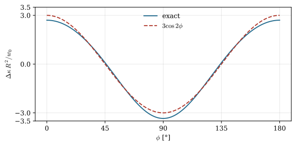
The two curves have the same shape, and the thin-ring result is off by about a tenth of the peak at this large deflection, \(w_0/R = 0.046\), where the bent wall is no longer a small change of a circle:
\[ \max|\Delta\kappa_\text{exact} - \Delta\kappa_\text{thin}| \,/\, (3w_0/R^2) =0.11 \]
Example 3: a printed and a steel flexspline
The printed strain wave gear of [2] has a flexspline of 50 teeth, module 1.5 mm, inside a circular spline of 52, a ratio of 25, and its wave generator pushes the wall out by 1.6 mm. The wall was 1.25 mm thick, and after the cup broke, 1.6 mm. Its mid-wall radius is about 35 mm (Figure 9.7.9). Find the bending strain of both walls, and compare it with a steel flexspline of the size of an industrial one, assumed here: 160 teeth of module 0.5 mm, \(R = 39.5\) mm, \(t = 0.6\) mm, \(E = 210\) GPa. How many stress cycles does each see in an hour at an input speed of 1000 rpm?
9.7.6 gives the strain, and each input turn gives two cycles.
Code
eps_pla = {t: 3*t*1.6/(2*35.0**2) for t in (1.25, 1.6)}
w0_steel = 0.5*(162 - 160)/2
eps_steel = 3*0.6*w0_steel/(2*39.5**2)
sigma_steel = 210e3*eps_steel                              # MPa
cycles_hour = 2*1000*60
The strains in per cent and the steel stress:
\[ \begin{aligned}\text{PLA},~t = 1.25:\quad \varepsilon &=0.245~\%,\quad t = 1.6:~\varepsilon =0.313~\%\\ \text{steel}:\quad \varepsilon &=0.0288~\%,\quad \sigma =60.6~\text{MPa}\\ \text{cycles per hour} &=120000\end{aligned} \]
The printed cup is bent about eight to eleven times harder than the steel one, 0.24 to 0.31 % against 0.03 %, because its teeth are three times larger for the same radius: the deflection is a module, and a printer cannot print fine teeth. The steel wall sees a modest 61 MPa, well below the fatigue limit of a spring steel. The PLA wall sees its strain 120 000 times an hour, fully reversed, and a thicker wall makes it worse, since the strain grows with \(t\): the test cup cracked, and a cup left bent overnight kept part of the ellipse, as PLA creeps at room temperature [2]. A longer cup helps, since the deflection then spreads over more length towards the bottom; a tougher, more flexible material helps more.
Which drive?
How To Mechatronics built and tested printed drives of each kind of this chapter and the last, and measured them the same way [2,7]. Their numbers are for PLA prints and a stepper motor, not for steel drives, but the trends are those of the designs:
| planetary, 2 stages | cycloidal | strain wave | belt, 2 stages | |
|---|---|---|---|---|
| ratio | 16 | 15 to 25 | 25 | 16 |
| efficiency | 0.78 to 0.95 | 0.6 to 0.66 | about 0.65 | 0.95 |
| backlash | 30 to 60′ | 60′ and more | small free play | 25′ |
| durability | 8 h test passed | worn after 2 h | flexspline broke | 8 h test passed |
| size | medium | most compact | long cup | medium |
The cycloidal drive was the most compact and carried 21.5 N·m before its discs deformed, but its many sliding contacts on printed surfaces cost efficiency and wore quickly. The printed strain wave gear had the least free play, as its preloaded mesh promises, and failed by the fatigue and creep of Example 3. The planetary gearbox, with ball bearings in the planets, and a two-stage GT2 belt drive did best overall. In steel the order changes: the cycloidal drive’s rolling pins carry shocks that would break gear teeth, and the strain wave gear’s zero backlash and low weight make it the standard drive of the wrist joints of industrial robots.
TipIn industry
Industrial robots use both drives of this chapter, bought as component sets or complete units. Cycloidal reducers, often with a planetary input stage in front of the cycloid stage, sit in the base, shoulder and elbow, where the torques and the shocks of a collision are largest. Strain wave gears sit in the wrist and in small robots, where weight and zero backlash count most. Both are chosen from catalogues by rated torque at a stated life, peak and emergency-stop torques, torsional stiffness and the lost motion near zero load, and the catalogue’s life calculation is that of the bearings: the eccentric bearings of the cycloid stage and the thin bearing of the wave generator.
Problems
Problem 1: Pins and lobes. A cycloidal drive of ratio \(-19\) is to have two discs. How many pins and lobes does it need, and does it work with two discs? What about \(-20\)?
Answer: 9.7.1: \(n - 1 = 19\) lobes and \(n = 20\) pins; 19 is odd, so two discs seat. A ratio of \(-20\) needs 20 lobes and 21 pins, an even number of lobes: one disc only, or two discs that are not identical.
Problem 2: The largest pin. For the drive of Figure 9.7.1 (\(n = 16\), \(R_m = 40\) mm, \(e = 1.5\) mm), how large may the pins be? Why are they not made that large?
Answer: \(r_p < \rho_\text{min} = 9.2\) mm. Long before that, neighbouring pins touch: they are \(2R_m\sin(\pi/n) = 15.6\) mm apart, so \(r_p < 7.8\) mm, and the disc between them gets thin valleys.
Problem 3: Strain wave ratio. A strain wave gear has a flexspline of 100 teeth. Find the ratio with the circular spline fixed, and with the flexspline fixed and the circular spline as output.
Answer: Circular spline fixed: \(i = -N_f/2 = -50\). Flexspline fixed: the Willis equation with \(\omega_f = 0\) gives \(\omega_c = \omega_w(1 - N_f/N_c) = 2\omega_w/102\), so \(i = 51\), in the same direction as the input.
Problem 4: A thinner flexspline. How thin must the wall of the printed flexspline of Example 3 be to bring the strain down to 0.1 %, and what is wrong with that?
Answer: \(t = 2\varepsilon R^2/(3w_0) = 2 \cdot 0.001 \cdot 35^2/(3 \cdot 1.6) = 0.51\) mm, a single extrusion line, under teeth of module 1.5 that carry the load; the wall would tear. Smaller teeth, and so a smaller \(w_0\), are the better way, and they need a finer printer or a moulded part.
Further reading
Braren’s patent [1] describes the cycloidal drive and its epitrochoid profile, and Blagojević et al. [3] analyse a two-stage design. Wang and Su [6] give the profile equations with the pin radius, the short width coefficient and its recommended values, and Sensinger [12] relates the profile to the stresses and the efficiency. Musser’s patent [8] and the application notes of Harmonic Drive [9,10] explain the strain wave gear. The videos of How To Mechatronics [2,7] show how both drives are designed, printed and tested.
References
[1]
Braren LK. Gear transmission. 1694031, 1928.
[2]
How To Mechatronics. Harmonic vs cycloidal drive: Torque, backlash and wear test 2022. https://www.youtube.com/watch?v=IXmCze1GsGU (accessed October 12, 2026).
[3]
Blagojevic M, Marjanovic N, Djordjevic Z, Stojanovic B, Disic A. A new design of a two-stage cycloidal speed reducer. Journal of Mechanical Design 2011;133. https://doi.org/10.1115/1.4004540.
[4]
Weisstein EW. Coin paradox n.d. https://mathworld.wolfram.com/CoinParadox.html (accessed October 12, 2026).
[5]
Weisstein EW. Epitrochoid n.d. https://mathworld.wolfram.com/Epitrochoid.html (accessed October 12, 2026).
[6]
Wang J, Su D. Active design method of tooth profiles for cycloid drive based on meshing efficiency. Transactions of Nanjing University of Aeronautics and Astronautics 2019;36:413–23. https://doi.org/10.16356/j.1005-1120.2019.03.005.
[7]
How To Mechatronics. Cycloidal vs belt vs planetary: The best 3D printed drive for your next robotic project? 2025. https://www.youtube.com/watch?v=9CDH4NMT_Pc (accessed October 12, 2026).
[8]
Musser CW. Strain wave gearing. 2906143, 1959.
[9]
Harmonic Drive LLC. Harmonic gear n.d. https://www.harmonicdrive.net/technology (accessed October 12, 2026).
[10]
Harmonic Drive LLC. Detailed operating principle n.d. https://legacy.harmonicdrive.net/reference/applicationnotes/principles.php (accessed October 12, 2026).
[11]
Harmonic Drive LLC. CSF-2A component sets n.d. https://www.harmonicdrive.net/products/component-sets/cup-type/csf-2a (accessed October 12, 2026).
[12]
Sensinger JW. Unified approach to cycloid drive profile, stress, and efficiency optimization. Journal of Mechanical Design 2010;132. https://doi.org/10.1115/1.4000832.