A car that stops from motorway speed has to get rid of more than half a megajoule in a few seconds, and its brakes do it by friction: pads or shoes press on a disc or a drum that turns with the wheel, and the friction turns the kinetic energy into heat. A clutchsv. koppling uses the same friction for the opposite purpose. It joins a turning shaft to one at rest, or at another speed, and slips until the two turn together, and the slip heats it in the same way. In both, the torque follows from the pressure on a friction surface, and the size follows from the heat that surface has to take.
The chapter starts with the disc brake, where the question of how the pressure spreads over a pad leads to the two classical assumptions, uniform pressure and uniform wear, and to the result that they give nearly the same torque. The energy of a stop and the temperature it gives the disc come next. The shoe brake and the band brake show what happens when the friction force has a moment about the pivot of the lever that applies the brake: the brake helps apply itself, and with enough friction it locks. The multi-plate clutch carries the disc brake’s result over to clutches, followed by the energy a clutch turns into heat while it engages, the cone clutch and the friction materials. Couplings that join shafts for good are the subject of the couplings chapter.
The disc brake
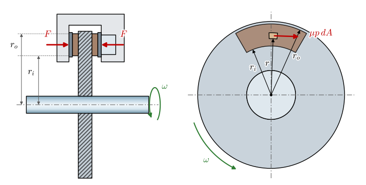
In a disc brakesv. skivbroms (Figure 9.15.1), a calipersv. bromsok straddles a disc that turns with the wheel. A hydraulic piston in the caliper presses one pad against the disc with the force \(F\), and the caliper, free to slide on its guide pins, pulls the other pad against the opposite face with the same force. Each pad covers a sector of the ring between the radii \(r_i\) and \(r_o\), over the angle \(\Delta\theta\). The disc slides under the pad, and at every point of the contact the pad pulls on the disc with the friction stress \(\mu p\), where \(p\) is the local contact pressure, against the disc’s motion.
Figure 9.15.1: A disc brake. Left: in section through the axis, the caliper presses the two pads against the faces of the disc with the force \(F\). Right: seen along the axis, the pad covers the ring from \(r_i\) to \(r_o\); on an element \(dA\) at the radius \(r\) the friction force \(\mu p\,dA\) acts against the disc’s rotation \(\omega\).
An element of the pad at the radius \(r\), of radial width \(dr\), spans the arc \(r\,\Delta\theta\) and has the area \(dA = r\,\Delta\theta\,dr\). It carries the normal force \(p\,dA\) and the friction force \(\mu p\,dA\), whose moment about the axis is \(r\mu p\,dA\). Summed over the pad,
where \(T_1\) is the torque of one pad on the disc. We write it as the friction force \(\mu F\) acting at an effective radius\(r_e\), \(T_1 = \mu F r_e\), and dividing the two integrals gives
The two pads act on both faces, so the braking torque on the disc is
\[
T = 2\mu F r_e
\tag{9.15.3}\]
The torque now depends on how the pressure is distributed over the pad, and equilibrium does not tell us. The pad and the disc are stiff, so the pressure depends on how well they fit, and the fit changes as they wear.
Uniform pressure and uniform wear
A new pad on a flat disc touches everywhere, and if both are stiff it presses equally hard everywhere: \(p\) is constant. This is the assumption of Example 5 of the Friction chapter, where it gave the torque of a clutch face, and 9.15.2 with a constant \(p\) gives
The pad does not stay new. The depth worn away grows with the pressure and with the distance slid, so the rate of wear is proportional to \(p\,v\), the wear law that Budynas and Nisbett use in their Section 16-5 [1]. On a disc the sliding speed \(v = r\omega\) grows with the radius, so the outer part of a new pad wears fastest. It wears until the pad has the shape in which it wears equally fast everywhere, and from then on \(p\,r\) is the same at every radius. The largest pressure \(p_a\) is at the inner radius, \(p = p_a r_i/r\), and 9.15.2 gives the mean radius,
\[
r_e = \frac{r_i + r_o}{2}
\tag{9.15.5}\]
A worn-insv. insliten brake carries its torque as if the whole friction force acted at the middle of the pad.
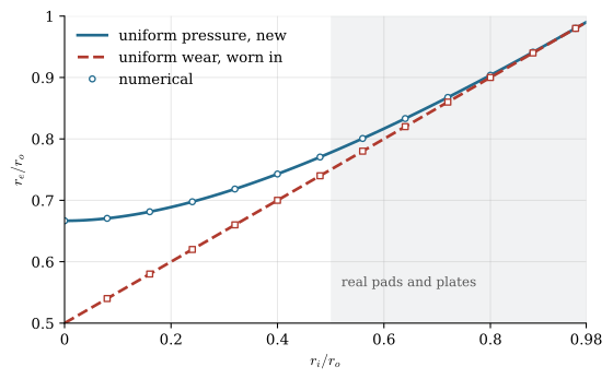
The two assumptions give nearly the same torque. Figure 9.15.2 compares them over the ratio \(r_i/r_o\), with both effective radii checked against a numerical integration of 9.15.2. For the proportions of real pads and clutch plates, \(r_i/r_o\) above 0.5, they differ by less than 4 %, and the worn-in value is the smaller. Every brake wears in, so the mean radius 9.15.5 is the one to design with.
Code
x = np.linspace(0.0, 0.98, 99) # r_i/r_o, with r_o = 1re_p =2/3*(1- x**3)/(1- x**2) # @eq-bc-re-pre_w = (1+ x)/2# @eq-bc-re-w# the same two radii from @eq-bc-re by numerical integration of the assumed pressuresdef re_numeric(xi, p_of_r): r = np.linspace(xi, 1.0, 2001) p = p_of_r(r)return np.trapezoid(p*r**2, r)/np.trapezoid(p*r, r)re_p_num = np.array([re_numeric(xi, lambda r: np.ones_like(r)) for xi in x])re_w_num = np.array([re_numeric(xi, lambda r, xi=xi: xi/r if xi >0else1/np.maximum(r, 1e-9)) for xi in x])assert np.allclose(re_p_num, re_p, rtol=1e-5)assert np.allclose(re_w_num[1:], re_w[1:], rtol=1e-5)diff_05 = (2/3*(1-0.5**3)/(1-0.5**2))/0.75-1# the difference at r_i/r_o = 0.5
Figure 9.15.2: The effective radius of a pad or a clutch ring as a fraction of its outer radius, for uniform pressure (9.15.4) and uniform wear (9.15.5); the markers integrate 9.15.2 numerically. In the shaded range the two differ by less than 4 %.
The energy of a stop
Whatever the brake, the energy it takes up is the kinetic energy of what it stops. A vehicle of mass \(m\) at the speed \(v\), and a rotor of moment of inertia \(J\) at the angular speed \(\omega\), carry
\[
E = \tfrac{1}{2}\,m v^2 + \tfrac{1}{2}\,J\omega^2
\tag{9.15.6}\]
The braking power at an instant is the torque times the angular speed, \(P = T\omega\), or the braking force times the speed. It is largest at the start of a stop and falls to zero with the speed. A hard stop lasts a few seconds, too short for the heat to leave the brake, so nearly all of \(E\) stays in the disc and the pads. With the specific heat capacity \(c\) and the mass \(m_d\) of the parts that take the heat, their mean temperature rises by
We write the temperature as \(\vartheta\) in this chapter, since \(T\) is the torque. Budynas and Nisbett, Section 16-9 [1], take \(c = 500\) J/(kg K) for steel and cast iron. The result is the mean temperature of the disc. The heat enters at the rubbing surfaces and needs several seconds to soak through the cast iron, so during the stop the surfaces run far hotter than the mean, and it is the surface temperature that the pad material has to survive.
Repeated stops
Between stops the disc cools by convection and radiation. In Newton’s model of cooling, the temperature above the surroundings \(\vartheta_\infty\) decays exponentially, \(\vartheta - \vartheta_\infty = (\vartheta_1 - \vartheta_\infty)\,e^{-\beta t}\) from the temperature \(\vartheta_1\), with \(\beta = hA/(m_d c)\) for the heat transfer coefficient \(h\) over the cooling area \(A\). A brake applied every \(t_1\) seconds settles into a cycle: each stop raises the temperature by \(\Delta\vartheta\) from its lowest value \(\vartheta_\min\) to its highest \(\vartheta_\max\), and the cooling over \(t_1\) brings it back down, \(\vartheta_\min - \vartheta_\infty = (\vartheta_\max - \vartheta_\infty)\,e^{-\beta t_1}\). Subtracting this from \(\vartheta_\max - \vartheta_\infty\) and setting \(\vartheta_\max - \vartheta_\min = \Delta\vartheta\) gives the highest temperature of the cycle
When the stops follow each other quickly, \(\beta t_1 \ll 1\), the denominator is small and the brake climbs to many times the temperature rise of one stop. The difficult quantity is \(h\), which depends on the speed of the air over the disc, on the ventilation and on the temperature itself, and Figure 16-24 of [1] gives curves for it.
Example 1: Stopping a car
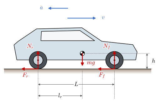
A car of \(m = 1500\) kg brakes from 100 km/h to rest with the deceleration \(a = 0.9g\), about what good tyres give on dry asphalt (Figure 9.15.3). Its centre of gravity lies \(h = 0.55\) m above the road and \(l_r = 0.58L\) ahead of the rear axle, so that 58 % of its weight rests on the front wheels, and the wheelbase is \(L = 2.7\) m. The tyres roll on the radius \(r_w = 0.31\) m. The front brakes have vented cast iron discs, 300 mm in diameter and 28 mm thick, pads from \(r_i = 100\) mm to \(r_o = 145\) mm with \(\mu = 0.4\), and one piston of 57 mm diameter in each caliper. Find the time and the distance of the stop, the clamp force and the brake fluid pressure at a front wheel, and the temperature rise of a front disc.
The car’s data are assumed, typical of a mid-size family car. The friction coefficient lies in the middle of the range Budynas and Nisbett give for molded disc brake pads in their Table 16-3 [1].
Figure 9.15.3: Example 1: a car braking from the speed \(v\) with the deceleration \(a\). The weight \(mg\) acts at the centre of gravity, \(h\) above the road and \(l_r\) ahead of the rear axle; the road carries the normal forces \(N_r\) and \(N_f\) and the braking forces \(F_r\) and \(F_f\).
The car decelerates without turning, so the forces on it give \(m\bm a\) and their moments about the centre of gravity vanish. With \(x\) forward and \(y\) up, and the moments taken anticlockwise,
\[
N_f = m g\,\frac{l_r}{L} + m a\,\frac{h}{L}
\tag{9.15.9}\]
Braking moves load from the rear axle to the front. The brakes are balanced when each axle brakes in proportion to the load it carries, so that front and rear tyres reach their grip at the same deceleration; then \(F_f = (N_f/mg)\,ma\). This is why the front discs of a car are larger than the rear ones. The braking force at one front tyre, \(F_f/2\), gives the wheel the torque \(T = r_w F_f/2\), which 9.15.3 with the worn-in radius 9.15.5 turns into the clamp force and the pressure in the caliper of piston diameter \(d_p\):
The stop lasts \(t_s = v_0/a\) over the distance \(s = v_0^2/(2a)\), and 9.15.6 gives the energy. The front axle takes the share \(N_f/mg\) of it, split over two discs. For the mass of a disc we take its friction ring, cast iron of \(\rho = 7200\) kg/m³ between the radii 85 mm and 150 mm, with 21 mm of solid metal through its thickness: two cheeks of 9 mm, and vanes that fill about 30 % of the 10 mm channel between them. The wheels’ own rotation adds about 3 % to the energy, which we neglect.
Code
m, v0, g =1500.0, 100/3.6, 9.81a_brake =0.9*gL_wb, h_cg, l_r =2.7, 0.55, 0.58*2.7r_w, r_i, r_o, mu, d_p =0.31, 0.100, 0.145, 0.4, 0.057share_f = l_r/L_wb + a_brake*h_cg/(g*L_wb) # N_f/(m g), @eq-bc-nfF_f = share_f*m*a_brake # braking force on the front axle [N]T_wheel = r_w*F_f/2# torque at one front wheel [N m]r_e = (r_i + r_o)/2F_clamp = T_wheel/(2*mu*r_e) # @eq-bc-disc solved for F [N]p_h = F_clamp/(np.pi*d_p**2/4) # brake fluid pressure [Pa]t_s, s_stop = v0/a_brake, v0**2/(2*a_brake)E_car =0.5*m*v0**2# @eq-bc-energy [J]E_disc = share_f*E_car/2# into one front disc [J]rho_ci, c_ci =7200.0, 500.0m_disc = rho_ci*np.pi*(0.150**2-0.085**2)*(2*0.009+0.3*0.010)dT_disc = E_disc/(m_disc*c_ci) # @eq-bc-temp [K]P_disc0 = F_f/2*v0 # braking power of one disc at the start [W]
The front axle carries a larger share of the load in the stop than at rest, and the stop takes
\[ \begin{aligned}N_f/mg &=0.7633,\quad t_s =3.146~\text{s},\quad s =43.7~\text{m}\\T &=1567.0~\text{N m},\quad F =15.99~\text{kN},\quad p_h =62.66~\text{bar}\end{aligned} \]
A front disc of \(m_d\) takes its share of the energy and warms by
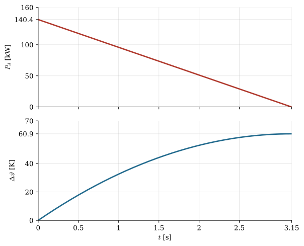
To check the energy balance we follow the stop in time. The speed falls linearly, \(v(t) = v_0 - a t\), the disc’s braking power is \(P_d(t) = (F_f/2)\,v(t)\), and its mean temperature rises as
which must end at the \(\Delta\vartheta\) above when the car stands still.
Code
t = np.linspace(0, t_s, 401)P_d = F_f/2*(v0 - a_brake*t) # braking power of one disc [W]E_t = np.concatenate([[0], np.cumsum(0.5*(P_d[1:] + P_d[:-1])*np.diff(t))])dT_t = E_t/(m_disc*c_ci)assertabs(dT_t[-1] - dT_disc) <1e-6*dT_disc # the work of friction is E_dfig, (ax1, ax2) = plt.subplots(2, 1, figsize=(6.4, 5.2), sharex=True)ax1.plot(t, P_d/1e3, color=RED, lw=2)ax1.set_ylabel('$P_d$ [kW]')ax1.set_ylim(0, 160)ax2.plot(t, dT_t, color=BLUE, lw=2)ax2.set_ylabel(r'$\Delta\vartheta$[K]')ax2.set_ylim(0, 70)ax2.set_xlabel('$t$ [s]')ax2.set_xlim(0, round(t_s, 2))for ax in (ax1, ax2): ax.grid(alpha=0.3)for s in ('top', 'right'): ax.spines[s].set_visible(False)end_ticks(ax1, y_extra=[round(P_disc0/1e3, 1)])end_ticks(ax2, x_extra=[], y_extra=[round(dT_disc, 1)])plt.tight_layout()plt.show()
Figure 9.15.4: The stop of Example 1 at one front disc: the braking power falls linearly with the speed from 140 kW, and the integrated heat raises the disc’s mean temperature by the value of 9.15.7.
The stop takes 3.1 s over 44 m, and the caliper presses the pads with 16 kN, which 63 bar of brake fluid pressure gives on the 57 mm piston; brake systems work at pressures of this order. The disc takes 220 kJ, and its mean temperature rises by about 60 K. That looks mild, but at the start of the stop the disc absorbs 140 kW, more than the engine of the car delivers, and the surfaces in contact with the pads run much hotter than the mean. A second and a third stop in quick succession add their 60 K each, less what the disc has shed in between, 9.15.8, and a car descending a mountain pass on its brakes heats them in the same way. The friction coefficient of most pad materials falls when they get hot, so the driver has to press harder for the same deceleration: the brakes fade.
The shoe brake
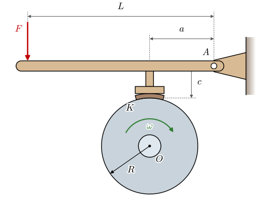
A shoe brakesv. backbroms presses a block lined with friction material against a drum by a lever (Figure 9.15.5). Its torque follows from the equilibrium of the lever, and where the pivot lies relative to the friction force matters a great deal.
Figure 9.15.5: Example 2: a shoe brake. The hand force \(F\) at the end of the lever presses the shoe on the drum at \(K\). The lever turns about the pin \(A\), at the distance \(a\) from the line of the normal force through \(K\) and \(O\), and \(c\) above the friction line, the tangent at \(K\).
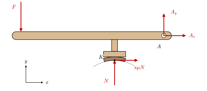
We take the shoe short, covering a small arc of the drum, so that the contact force acts at one point \(K\): the normal force \(N\) along the line through the drum’s centre, and the friction force along the tangent (Figure 9.15.6). The drum’s surface slides under the shoe and drags it along, so the friction force on the shoe points the way the surface moves. We write it \(s\mu N\) along \(x\), with \(s = +1\) when the drum turns clockwise and \(s = -1\) when it turns anticlockwise. The moment equation about the pivot \(A\) leaves out the pin force,
\[
F L - N a + s\mu N c = 0
\quad\Rightarrow\quad
N = \frac{F L}{a - s\mu c}
\tag{9.15.10}\]
and the braking torque on the drum is \(T = \mu N R\).
Figure 9.15.6: Example 2: the lever and its shoe, freed from the drum and from the pin \(A\). The drum pushes on the shoe at \(K\) with \(N\) and drags it with the friction \(s\mu N\); \(s = +1\) for a drum turning clockwise.
With the pivot on the friction line, \(c = 0\), the friction force has no moment about \(A\), \(N = FL/a\) and \(T = \mu F R\,L/a\): the lever’s ratio times the friction. With the pivot above the friction line and the drum turning clockwise, the friction force turns the lever the same way as the hand force, presses the shoe harder and raises \(N\). The brake is self-energizingsv. självförstärkande. Turning the other way, the friction lifts the shoe, and the brake is de-energizing. As \(\mu c\) approaches \(a\) the denominator vanishes, and a brake that needs no hand force locks at the slightest touch. The brake is self-lockingsv. självlåsande for
\[
\mu \ge \frac{a}{c}
\tag{9.15.11}\]
Budynas and Nisbett, Section 16-1 [1], arrive at the same condition for a doorstop whose pad has a finite length, with \(c\) measured to the pad’s centre of pressure. The printed brake of Example 7 in the Friction chapter is this mechanism: its denominator \(20 - s\mu\,d/2\) is \(a - s\mu c\) with \(a = 20\) mm and \(c = d/2 = 4\) mm, and with an offset that small the self-energizing changed the braking moment by only 7 %.
Self-energizing has a price. With \(c > 0\) the torque grows as \(\mu/(1 - \mu c/a)\), faster than \(\mu\), so when the friction coefficient drops with heat or water, the torque drops more than in proportion. Budynas and Nisbett, Section 16-6 [1], note that a 30 % loss of friction, not unusual in a hot or wet drum brake, can call for 50 % more pedal force, and that a disc brake, with no self-energizing at all, is far less sensitive. The shoes of a car’s drum brake cover 90° to 120° of the drum, and then the pressure varies along the shoe and the torque is the integral \(T = \int \mu\,p(\varphi)\,b R^2\,d\varphi\) over the lining of width \(b\). Budynas and Nisbett treat these long shoes in their Sections 16-2 and 16-3; the conclusions about self-energizing and self-locking are the same.
Example 2: A lever shoe brake
The shoe brake of Figure 9.15.5 holds a winch drum of radius \(R = 150\) mm. The lever has \(L = 600\) mm, \(a = 200\) mm and \(c = 100\) mm, the hand pushes with \(F = 150\) N, and the lining has \(\mu = 0.4\). Find the braking torque for both directions of rotation, and for the pivot moved onto the friction line. A designer wants more torque from the same hand and proposes to raise the pivot to \(c = 400\) mm. What happens when the lining’s friction coefficient drifts with temperature and moisture between 0.3 and 0.5?
9.15.10 gives \(N\) for each case and \(T = \mu N R\) the torque; the lock follows from 9.15.11.
Code
R_d, L_l, a_l, F_h, mu_s =0.150, 0.600, 0.200, 150.0, 0.4def shoe_torque(mu, c, s):# @eq-bc-shoe and T = mu N R; s = +1 clockwise (self-energizing for c > 0) N = F_h*L_l/(a_l - s*mu*c)return mu*N*R_dT_cw, T_ccw, T_0 = shoe_torque(mu_s, 0.1, 1), shoe_torque(mu_s, 0.1, -1), shoe_torque(mu_s, 0.0, 1)mu_lock_100, mu_lock_400 = a_l/0.1, a_l/0.4# @eq-bc-lockT_400 = {mu: shoe_torque(mu, 0.4, 1) for mu in (0.3, 0.4, 0.45)}
The offset of 100 mm makes the brake half as strong again in one direction as in the other:
\[ \begin{aligned}s = +1:\quad T &=33.8~\text{N m}\\s = -1:\quad T &=22.5~\text{N m}\\c = 0:\quad T &=27.0~\text{N m},\quad \mu_\text{lock} = a/c =2.0\end{aligned} \]
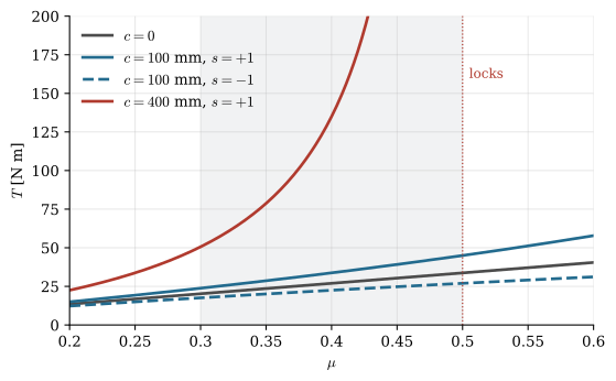
With \(c = 100\) mm the brake locks only at \(\mu = 2\), which no lining reaches. Raising the pivot to \(c = 400\) mm brings the lock down to \(\mu = a/c = 0.5\), inside the range the lining drifts over. Figure 9.15.7 shows the torque against the friction coefficient: at \(\mu = 0.4\) the raised pivot gives the designer the torque
Figure 9.15.7: The braking torque of Example 2 against the friction coefficient. The shaded band is the drift of the lining. The raised pivot (\(c = 400\) mm) multiplies the torque, but across the band the torque grows without bound, and the brake locks at \(\mu = 0.5\).
At \(\mu = 0.4\) the raised pivot gives 135 N m against 34 N m with the original lever, four times more for the same hand. Over the band of friction coefficients, though, its torque runs from 51 N m to infinity, and somewhere near the top of the band the drum stops dead the moment the shoe touches. The original lever, with its torque between 24 and 45 N m, behaves almost like the neutral one. A self-energizing gain of 1.25, the ratio \(a/(a - \mu c)\) at \(c = 100\) mm, is a reasonable design; a gain of 5 is a brake whose torque nobody controls.
The band brake
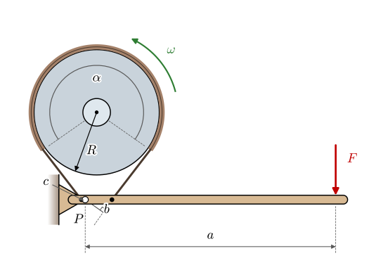
A band brakesv. bandbroms wraps a steel band, lined with friction material, the angle \(\alpha\) around a drum (Figure 9.15.8). The band is the rope of the capstan in Example 4 of the Friction chapter, where 5.6.3 showed that the tension grows exponentially along the wrap when the band slides. Between the slack end, with the tension \(F_1\), and the tight end, \(F_2\),
\[
F_2 = F_1\,e^{\mu\alpha}
\tag{9.15.12}\]
The drum drags the band along with its surface, so the tight end is the end toward which the surface moves. The difference of the two tensions acts at the radius \(R\) and gives the braking torque,
The capstan derivation also gives the pressure. A band element \(d\theta\) under the tension \(F\) presses on the drum with \(dN = F\,d\theta\), over the area \(wR\,d\theta\) of a band of width \(w\), so
\[
p = \frac{F}{wR}
\tag{9.15.14}\]
The pressure follows the tension, growing exponentially from the slack end to the tight end, where it is largest, \(p_\max = F_2/(wR)\), Eq. 16-22 in [1]. The lining wears fastest at the tight end.
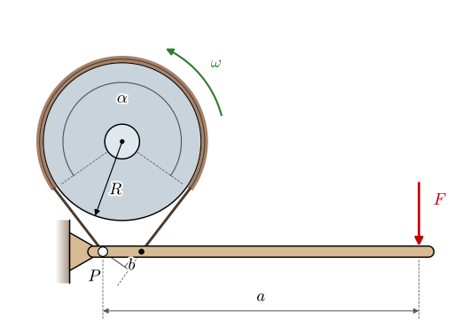
How the two tensions arise depends on how the band’s ends are fastened to the lever. In the simple band brake (Figure 9.15.8 (a)), one end is anchored at the lever’s pivot \(P\), so its tension has no moment about \(P\). The other end pulls on the lever with the perpendicular arm \(b\), and the hand force \(F\) at the arm \(a\) balances it, \(Fa = F_b b\). When the drum turns so that the end at \(b\) is the slack end, anticlockwise in the figure, \(F_1 = Fa/b\) and 9.15.13 gives
\[
T = F R\,\frac{a}{b}\left(e^{\mu\alpha} - 1\right)
\tag{9.15.15}\]
When the drum turns the other way, the end at \(b\) is the tight end, \(F_2 = Fa/b\), and the torque is smaller by the factor \(e^{\mu\alpha}\). A brake that must hold equally in both directions fastens both ends to the lever at the same arm \(b\) on the same side of the pivot, the summing band brake: then \(Fa = (F_1 + F_2)\,b\) and \(T = FR\,(a/b)\,(e^{\mu\alpha} - 1)/(e^{\mu\alpha} + 1)\) either way.
In the differential band brake (Figure 9.15.8 (b)), the pivot sits between the two ends. The slack end at the arm \(b\) resists the hand force, and the tight end at the arm \(c\) on the other side of the pivot helps it. The moments about \(P\) give \(Fa = F_1 b - F_2 c = F_1\,(b - c\,e^{\mu\alpha})\), and
\[
T = \frac{F R\,a\left(e^{\mu\alpha} - 1\right)}{b - c\,e^{\mu\alpha}}
\tag{9.15.16}\]
The tight end does part of the work, so a small hand force gives a large torque. With \(c = 0\) the formula is that of the simple brake. When \(c\,e^{\mu\alpha}\) reaches \(b\), the tight end alone holds the lever down: the differential band brake is self-locking for
Figure 9.15.8: Example 3: two band brakes. (a) The simple band brake, one end anchored at the pivot \(P\), the other at the perpendicular arm \(b\). (b) The differential band brake, the pivot between the ends, at the arms \(c\) and \(b\). The band wraps the angle \(\alpha\); with the drum turning anticlockwise the left end is the tight end.
Example 3: Band brakes on a drum
The band brakes of Figure 9.15.8 act on a drum of radius \(R = 200\) mm with \(\alpha = 250°\) of wrap and a band \(w = 60\) mm wide, lined with a woven lining of \(\mu = 0.35\). The levers have \(a = 800\) mm. The simple brake has \(b = 80\) mm, the differential brake \(b = 70\) mm and \(c = 10\) mm. Find the torque of the simple brake in both directions for \(F = 150\) N, and the largest lining pressure, which should stay below the 690 kPa that Budynas and Nisbett give for woven linings in their Table 16-4 [1]. What hand force does the differential brake need for the same torque, and at what friction coefficient does it lock?
9.15.15 gives the torque with the end at \(b\) slack, and the tensions with 9.15.12 give the pressure 9.15.14. For the reverse direction \(F_2 = Fa/b\). The differential brake’s hand force follows from 9.15.16 solved for \(F\), and its lock from 9.15.17.
Code
R_b, w_b, alpha, mu_b =0.200, 0.060, np.radians(250), 0.35a_b, F_b =0.800, 150.0b_s =0.080# simple brakeb_d, c_d =0.070, 0.010# differential brakee_ma = np.exp(mu_b*alpha)F1 = F_b*a_b/b_s # end at b slackF2 = F1*e_ma # @eq-bc-bandT_simple = (F2 - F1)*R_b # @eq-bc-band-torquep_max = F2/(w_b*R_b) # @eq-bc-band-p at the tight endF2_rev = F_b*a_b/b_s # drum reversed: end at b tightT_rev = (F2_rev - F2_rev/e_ma)*R_bF_diff = T_simple*(b_d - c_d*e_ma)/(R_b*a_b*(e_ma -1)) # @eq-bc-band-diff for FF2_diff = F_diff*a_b/(b_d - c_d*e_ma)*e_mamu_lock = np.log(b_d/c_d)/alpha # @eq-bc-band-lock
The simple brake holds far more in one direction than the other, and its lining pressure stays within the limit:
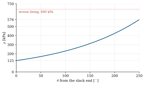
To check 9.15.13 against the pressure, we integrate the friction stress of 9.15.14 over the lining, with the tension \(F(\theta) = F_1 e^{\mu\theta}\) measured from the slack end,
\[
T = \int_0^\alpha \mu\,p(\theta)\,w R^2\,d\theta
\]
which must equal \((F_2 - F_1)R\).
Code
th = np.linspace(0, alpha, 1001)p_th = F1*np.exp(mu_b*th)/(w_b*R_b) # @eq-bc-band-p along the wrap [Pa]T_int = np.trapezoid(mu_b*p_th*w_b*R_b**2, th)assertabs(T_int - T_simple) <1e-4*T_simplefig, ax = plt.subplots(figsize=(6.4, 3.6))ax.plot(np.degrees(th), p_th/1e3, color=BLUE, lw=2)ax.axhline(690, color=RED, lw=0.9, ls=':')ax.text(5, 650, 'woven lining, 690 kPa', color=RED, fontsize=9)ax.set_xlim(0, 250)ax.set_ylim(0, 750)ax.set_xlabel(r'$\theta$ from the slack end [$^\circ$]')ax.set_ylabel('$p$ [kPa]')ax.grid(alpha=0.3)for s in ('top', 'right'): ax.spines[s].set_visible(False)end_ticks(ax, y_extra=[round(p_th[0]/1e3), round(p_th[-1]/1e3)])plt.show()
Figure 9.15.9: The lining pressure of the simple band brake in Example 3, from the slack end to the tight end. Its integral, weighted with \(\mu w R^2\), reproduces the torque of 9.15.13.
The integral agrees with \((F_2 - F_1)R\), and the pressure rises 4.6 times along the wrap, from 125 kPa to 576 kPa. Reversed, the simple brake holds only 235 N m. The differential brake needs 45 N instead of 150 N for the same 1080 N m, a third of the hand force, because the tight end pulls the lever on with \(c\,F_2\). But it locks at \(\mu = 0.45\), and Table 16-4 of [1] gives 0.45 as the mean friction coefficient of a woven lining; a lining a little grippier than ours, or ours on a cold dry morning, would lock the drum. In a differential brake meant to be worked by hand, \(b\) must stay well above \(c\,e^{\mu\alpha}\) for the highest friction coefficient the lining can reach.
Multi-plate clutches
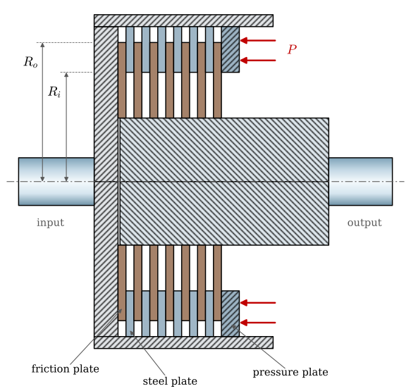
A friction clutch joins two shafts by pressing friction surfaces together, and it can be engaged and released while they turn. The disc brake’s analysis carries over: a full ring from \(R_i\) to \(R_o\), pressed by the axial force \(P\), carries on each friction surface the torque \(\mu P r_e\), with the effective radius of 9.15.5 or 9.15.4. The clutch of a car with a manual gearbox has one disc lined on both faces, clamped between the engine’s flywheel and a pressure plate, so it has two friction surfaces. Where more torque must fit in a small diameter, as in motorcycles, automatic gearboxes and machine tools, a multi-plate clutchsv. lamellkoppling (Figure 9.15.10) stacks plates that are keyed in turn to an outer basket and to an inner hub. One axial force \(P\) presses the whole stack, so every friction surface carries the same normal force, if we neglect the friction of the plates on their splines. With \(n\) friction surfaces the slip torquesv. slirmoment is
\[
T = n\,\mu P r_e
\tag{9.15.18}\]
With the worn-in radius of 9.15.5, \(T = n\mu P\,(R_i + R_o)/2\). A clutch that runs in oil, a wet clutch, has its heat carried away by the oil and wears little, but the oil lowers the friction coefficient to around 0.1, so it needs more plates than a dry one.
Figure 9.15.10: Example 4: a multi-plate clutch in section. Seven friction plates (brown) on the splines of the hub alternate with six steel plates keyed to the basket; springs press the pressure plate with the force \(P\), and the stack has \(n = 14\) friction surfaces between the radii \(R_i\) and \(R_o\).
Engaging a clutch
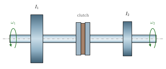
A clutch that closes between two shafts turning at different speeds slips until they turn together. Take two inertias \(I_1\) and \(I_2\) at \(\omega_1 > \omega_2\) (Figure 9.15.11), joined by a clutch that slips with the constant torque \(T\), and no other torque on them. The clutch slows the first and speeds up the second,
\[
I_1\dot\omega_1 = -T,\qquad I_2\dot\omega_2 = T
\]
so the slip speed \(\omega_1 - \omega_2\) falls at the constant rate \(T\,(1/I_1 + 1/I_2)\) and vanishes after the time
Figure 9.15.11: Two inertias joined by a clutch. The clutch slips with the torque \(T\) until \(\omega_1\) and \(\omega_2\) are equal.
The friction power is the torque times the slip speed, which falls linearly to zero, so the energy turned into heat is half of \(T(\omega_1 - \omega_2)\,t_s\). Budynas and Nisbett, Section 16-8 [1], insert 9.15.19 to get
\[
E = \frac{I_1 I_2\,(\omega_1 - \omega_2)^2}{2\,(I_1 + I_2)}
\tag{9.15.20}\]
The clutch torque has dropped out. A gentle clutch slips longer at a lower torque and turns exactly as much energy into heat as a sharp one. The engagement conserves the angular momentum \(I_1\omega_1 + I_2\omega_2\) but not the kinetic energy, like a perfectly plastic collision, and \(E\) is the kinetic energy lost. When the driving side is held at its speed by its motor, as an engine is by its throttle, the limit \(I_1 \to \infty\) applies and \(E = \tfrac12 I_2(\omega_1 - \omega_2)^2\): starting a load from rest turns into heat exactly the kinetic energy that the load receives.
Example 4: The clutch of a motorcycle
A motorcycle’s wet multi-plate clutch (Figure 9.15.10) has seven friction plates, so \(n = 14\), lined between \(R_i = 55\) mm and \(R_o = 70\) mm, with \(\mu = 0.12\) in oil; Budynas and Nisbett list 0.09 to 0.15 for resilient paper running wet in their Table 16-3 [1]. Its springs press the stack with \(P = 1.5\) kN. The engine gives at most 65 N m and drives the clutch basket through a primary reduction of 2.0.
Find the slip torque under both pressure assumptions and the margin against slip.
The rider starts off in first gear, with the ratio 8.1 from the clutch to the rear wheel and a wheel of radius 0.30 m, holding the engine at 3000 rpm while the clutch slips. Machine and rider weigh 280 kg. How much heat goes into the clutch, and how warm do its steel plates get if they keep it, at about 0.6 kg together?
The data are assumed, of the size found in mid-size motorcycles. For (a), 9.15.18 with the two effective radii, and the largest pressure of the worn-in clutch from 9.15.1 with \(\Delta\theta = 2\pi\) and \(p = p_a R_i/r\), \(P = 2\pi p_a R_i (R_o - R_i)\). For (b), the engine side is held at its speed, so 9.15.20 in the limit \(I_1 \to \infty\) applies, with the motorcycle’s mass seen at the clutch as the inertia \(I_2 = m\,(r_w/i)^2\) for the ratio \(i = 8.1\). The slip ends when the clutch hub turns at the basket’s speed \(\omega_c = \omega_e/2\), with the motorcycle at \(v = \omega_c r_w/i\), and \(E = \tfrac12 I_2\omega_c^2 = \tfrac12 m v^2\).
\[ \begin{aligned}I_2 &=0.384~\text{kg m}^2,\quad v =20.9~\text{km/h}\\E &=4.74~\text{kJ},\quad \Delta\vartheta =15.8~\text{K}\end{aligned} \]
The uniform-pressure torque is 0.5 % above the worn-in one, since the ring is narrow, \(R_i/R_o = 0.79\). The margin of 1.21 is small on purpose: a motorcycle clutch is made to slip under a torque shock, and the rider has to pull the lever against the springs at every gear change, so the springs are no stronger than they must be. The largest pressure of 290 kPa is a tenth of what Table 16-3 allows for wet paper. The slip stops at 21 km/h, and the clutch turns 4.7 kJ into heat whether the rider lets it in gently or not.
We test that last claim by integrating the engagement in time. With the clutch torque \(T(t)\) chosen by the rider’s hand, the hub speeds up by \(I_2\dot\omega_2 = T(t)\) until \(\omega_2 = \omega_c\), and the heat is
\[
E = \int_0^{t_s} T(t)\,\big(\omega_c - \omega_2(t)\big)\,dt
\]
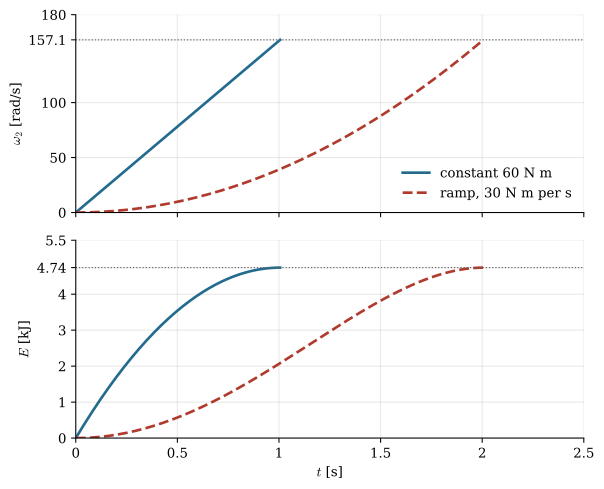
We try a constant 60 N m and a lever let out slowly, the torque rising linearly by 30 N m per second.
Code
def engage(T_of_t, dt=1e-4):# integrate I_2 w2' = T(t) until the hub reaches the basket; return t, w2, heat so far t, w2, E = [0.0], [0.0], [0.0]while w2[-1] < w_c: T_now = T_of_t(t[-1]) E.append(E[-1] + T_now*(w_c - w2[-1])*dt) w2.append(w2[-1] + T_now/I_2*dt) t.append(t[-1] + dt)return np.array(t), np.array(w2), np.array(E)runs = {'constant 60 N m': engage(lambda t: 60.0),'ramp, 30 N m per s': engage(lambda t: 30.0*t)}for t_r, w_r, E_r in runs.values():assertabs(E_r[-1] - E_slip) <0.01*E_slip # the heat does not depend on T(t)fig, (ax1, ax2) = plt.subplots(2, 1, figsize=(6.4, 5.2), sharex=True)for (lab, (t_r, w_r, E_r)), col, ls inzip(runs.items(), (BLUE, RED), ('-', '--')): ax1.plot(t_r, w_r, color=col, lw=2, ls=ls, label=lab) ax2.plot(t_r, E_r/1e3, color=col, lw=2, ls=ls)ax1.axhline(w_c, color='0.4', lw=0.9, ls=':')ax2.axhline(E_slip/1e3, color='0.4', lw=0.9, ls=':')ax1.set_ylabel(r'$\omega_2$[rad/s]')ax1.set_ylim(0, 180)ax2.set_ylabel('$E$ [kJ]')ax2.set_ylim(0, 5.5)ax2.set_xlabel('$t$ [s]')ax2.set_xlim(0, 2.5)ax1.legend(frameon=False, loc='lower right')for ax in (ax1, ax2): ax.grid(alpha=0.3)for s in ('top', 'right'): ax.spines[s].set_visible(False)end_ticks(ax1, y_extra=[round(w_c, 1)])end_ticks(ax2, y_extra=[round(E_slip/1e3, 2)])plt.tight_layout()plt.show()
Figure 9.15.12: The start of Example 4 integrated in time, for a constant clutch torque and for a lever let out slowly. Top: the speed of the clutch hub rising to the basket’s speed (dotted). Bottom: the heat in the clutch, which ends at \(\tfrac12 I_2\omega_c^2\) (dotted) in both cases.
The slow start takes twice as long and ends with the same 4.7 kJ, to within the time step. If the 0.6 kg of steel plates kept it all they would warm by 16 K; in fact the oil carries most of it away. One start is harmless. A rider who slips the clutch for minutes in a queue feeds it heat continuously, and the oil temperature then decides.
Cone clutches
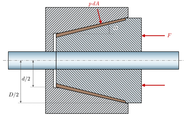
In a cone clutch (Figure 9.15.13) the friction surfaces are cones. A cone on one shaft slides into a cup on the other, both inclined at the half angle \(\alpha\) to the axis, and the axial force \(F\) presses them together.
Figure 9.15.13: A cone clutch in section. The cup on the left shaft and the lined cone on the right shaft meet on a cone of half angle \(\alpha\) between the diameters \(d\) and \(D\); the axial force \(F\) presses them together, and the pressure \(p\) acts normal to the cone.
A ring of the contact between the radii \(r\) and \(r + dr\) has the slant width \(dr/\sin\alpha\), so its area is \(dA = 2\pi r\,dr/\sin\alpha\). The pressure acts normal to the cone. Its axial component \(p\,dA\sin\alpha = 2\pi p\,r\,dr\) is the same as for a flat ring between the same radii, so the axial force is that of a flat clutch. The friction force \(\mu p\,dA\) acts along the circumference with the arm \(r\), on an area that is larger by \(1/\sin\alpha\), and
\[
T = \frac{\mu F r_e}{\sin\alpha}
\tag{9.15.21}\]
with \(r_e = (D + d)/4\) worn in, 9.15.5. A cone of \(\alpha = 12°\) carries 4.8 times the torque of a flat ring with the same axial force. The wedge has its price on release: below about 8° the cone sticks in the cup and takes a large force to pull out, and Budynas and Nisbett, Section 16-7 [1], recommend 10° to 15°. The synchronizers of a manual gearbox are small cone clutches: before the dog teeth of a gear engage, a ring with a conical face rubs on a cone of the gear and brings the two to the same speed.
Friction materials
A friction material should have a high friction coefficient that stays the same over the temperature, the speed, the pressure and the moisture it meets, survive the temperatures of hard stops, wear slowly without scoring the disc, and conduct the heat away from the surface. No material does all of it, and the choice depends on the duty. Most pads and linings are organic: fibres, fillers and friction modifiers bound in a phenolic resin and moulded. For decades the fibre was asbestos, which the EU banned in 2005; today it is aramid, glass, mineral or steel fibre, and pads with much steel fibre are called semi-metallic. Sintered metal pads, copper and iron powder with friction modifiers pressed and sintered, take more heat and pressure and serve in heavy-duty clutches, motorcycles and trains; with a substantial ceramic content they are called cermets. Wet clutches use paper-based or sintered linings in oil.
Table 9.15.1 collects a few of them from Budynas and Nisbett’s Table 16-3 [1], in SI units. The continuous temperature is what the material takes in steady service, the instantaneous what it survives for a moment, the surface of a hard stop in Figure 9.15.4. Above the continuous temperature the friction coefficient of an organic material falls, the fade of Example 1, and the resin starts to decompose.
Table 9.15.1: Friction materials for brakes and clutches, converted to SI from Table 16-3 of Budynas and Nisbett [1].
Material
\(\mu\)
\(p_\max\) [MPa]
\(\vartheta_\max\), instantaneous [°C]
\(\vartheta_\max\), continuous [°C]
Use
Rigid molded, non-asbestos (dry)
0.33–0.63
0.7–1.0
260–400
clutches and brakes
Sintered metal (dry)
0.29–0.33
2.1–2.8
500–550
300–350
clutches, caliper disc brakes
Cermet (dry)
0.32
1.0
815
400
brakes and clutches
Sintered metal (wet)
0.06–0.08
3.4
500
300
clutches
Resilient paper (wet)
0.09–0.15
2.8
150
clutches, transmission bands
Woven cotton
0.47
0.69
110
77
industrial clutches and brakes
A printed part makes a poor friction material. The PLA of the servo brake in the Friction chapter softens near its glass transition at about 60 °C, so a printed brake can hold a shaft or slip briefly, and a brake that slips for long needs a lining of one of the materials above, glued or clipped onto the printed lever.
TipIn industry: brakes are rated by torque and by heat
Industrial brakes and clutches are bought from catalogues, which give for each size the torque and two thermal limits: the energy one engagement may turn into heat, and the power the unit can shed continuously, which sets how many engagements per hour it takes. The designer checks the torque with a service factor, as for couplings, and the heat with 9.15.20 or 9.15.6. Holding brakes on hoists, lifts and robot joints are fail-safe: springs apply them and a magnet or hydraulic pressure releases them, so that a power failure sets the brake. Car brake pads are developed on brake dynamometers, and a pad carries on its edge a two-letter code by SAE J866 for its friction coefficient when cold and when hot, E for 0.25 to 0.35, F for 0.35 to 0.45 and G for 0.45 to 0.55. Since Euro 7, Regulation (EU) 2024/1257, the particles that a car’s brakes give off are limited as well, to 7 mg/km of PM10 for most cars and 3 mg/km for purely electric ones, which drives the development of pad materials and coated discs that wear less.
Problems
Problem 1: A new pad. Redo the clamp force of Example 1 with the uniform-pressure radius of a new pad (Figure 9.15.14). Below what ratio \(r_i/r_o\) do the two assumptions differ by more than 5 %?
Figure 9.15.14: The disc brake of Problem 1, as in Example 1.
Answer:9.15.4 gives \(r_e = 123.9\) mm against 122.5 mm, so the new pad needs 1.1 % less clamp force, 15.8 kN instead of 16.0 kN. The ratio of 9.15.4 to 9.15.5 exceeds 1.05 for \(r_i/r_o < 0.44\).
Problem 2: Repeated stops. The car of Example 1 (Figure 9.15.15) repeats its stop from 100 km/h every 60 s, a brake fade test. Take \(\beta = 0.007\) s\(^{-1}\) for the cooling of a front disc, an ambient temperature of 20 °C, and neglect the cooling during the stops and the time it takes to get back up to speed. What are the highest and lowest mean disc temperatures once the cycle has settled?
Figure 9.15.15: The car of Problem 2.
Answer:9.15.8 with \(\Delta\vartheta = 61\) K and \(\beta t_1 = 0.42\) gives \(\vartheta_\max = 20 + 61/(1 - e^{-0.42}) = 198\) °C and \(\vartheta_\min = 137\) °C, three times the rise of one stop. The surfaces run hotter still.
Problem 3: Holding a load. The shoe brake of Example 2 (Figure 9.15.16), with \(c = 100\) mm and \(\mu = 0.4\), must hold a winch drum on which the load pulls with 40 N m. What hand force does it take when the load turns the drum clockwise, and when it turns it anticlockwise? Which way should the winch be mounted?
Figure 9.15.16: The shoe brake of Problem 3.
Answer:\(N = T/(\mu R) = 667\) N, and 9.15.10 gives \(F = N(a - s\mu c)/L\): 178 N clockwise (\(s = +1\)), 267 N anticlockwise. Mount it so that the load turns the drum clockwise, where the brake is self-energizing.
Problem 4: Both directions. The drum of Example 3 needs a brake that holds the same in both directions. Find the torque of a summing band brake with both ends at \(b = 80\) mm, \(a = 800\) mm and \(F = 150\) N, and compare it with the simple brake (Figure 9.15.17).
Figure 9.15.17: The simple band brake of Example 3; in Problem 4 its anchored end moves out to the arm \(b\) as well.
Answer:\(Fa = (F_1 + F_2)b\) gives \(F_1 + F_2 = 1500\) N, and with \(e^{\mu\alpha} = 4.61\), \(T = FR\,(a/b)(e^{\mu\alpha} - 1)/(e^{\mu\alpha} + 1) = 193\) N m in either direction, between the simple brake’s 235 N m and 1082 N m.
Problem 5: Engaging two free inertias. A clutch joins a motor’s rotor and flywheel, \(I_1 = 0.5\) kg m² at 1450 rpm with the motor switched off, to a machine of \(I_2 = 1.5\) kg m² at rest (Figure 9.15.18). It slips with 100 N m. Find the slip time, the common final speed and the heat.
Figure 9.15.18: The two inertias of Problem 5.
Answer:9.15.19 gives \(t_s = 0.57\) s. The angular momentum is kept, so the final speed is \(I_1\omega_1/(I_1 + I_2) = 362\) rpm, and 9.15.20 gives \(E = 4.3\) kJ, three quarters of the flywheel’s 5.8 kJ.
Further reading
Budynas and Nisbett [1] cover brakes and clutches in their Chapter 16: the long-shoe drum brakes left out here, band and disc brakes, cone clutches, the energy and temperature of braking and tables of friction materials. Limpert [2] treats the brakes of cars and trucks in depth, from the braking force distribution between the axles to the temperature of discs and drums. Mägi, Melkersson and Evertsson [3] cover brakes and clutches in Swedish. Couplings that join shafts permanently, and the catalogue practice for choosing them, are in the couplings chapter.