“The formula shows, what is indeed clear à priori, that the notion of the inverse or reciprocal matrix fails altogether when the determinant vanishes: the matrix is in this case said to be indeterminate.”
— Arthur Cayley, A memoir on the theory of matrices, 1858
A square matrix \(\bm A\) maps the plane onto itself (Chapter 3.10). The determinant \(\det\bm A\) measures how much the map scales areas, and the inverse \(\bm A^{-1}\) undoes the map. Cayley’s sentence ties the two together: a map can be undone exactly when its area factor differs from zero.
The determinant as an area factor
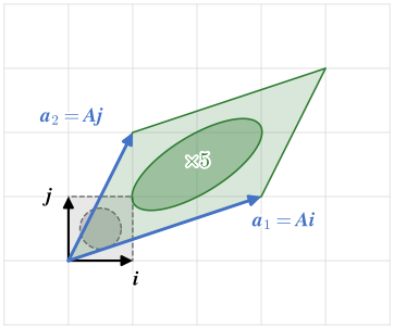
The columns of a \(2\times 2\) matrix \(\bm A = [\bm a_1\ \bm a_2]\) are the images of \(\bm i\) and \(\bm j\). The unit square spanned by \(\bm i\) and \(\bm j\) therefore lands on the parallelogram spanned by \(\bm a_1\) and \(\bm a_2\), and in Chapter 3.7 we found the signed area of that parallelogram to be the determinant of the matrix with the two vectors as columns,
The unit square has area \(1\), so its image has area \(|\det\bm A|\). The same holds for every other region. A linear map keeps the grid lines straight, parallel and evenly spaced, so each small square of the grid lands on a copy of one and the same parallelogram, scaled by the same factor. A region covered by many small squares, a disk say, has its area multiplied by that factor too.
A map \(\bm x\mapsto\bm A\bm x\) multiplies every area by \(|\det\bm A|\).
The video plays the matrix \(\bm A = \begin{bmatrix} 3 & 1\\ 1 & 2\end{bmatrix}\) on the plane. The unit square and a disk to its left are mapped together, and the ratio of the areas of the disk and its image, computed from the mapped outline, matches \(\det\bm A = 5\) at every instant.
Example 1: Area factor of a map
Figure 3.11.1: The matrix \(\bm A\) carries the unit square to the parallelogram of its columns \(\bm a_1\) and \(\bm a_2\), and the disk inside the square to an ellipse inside the parallelogram.
The matrix \(\bm A = \begin{bmatrix} 3 & 1\\ 1 & 2\end{bmatrix}\) maps the unit square and the disk of radius \(r = 0.32\) centred in it, Figure 3.11.1. Find the areas of the two images.
so the parallelogram has the area \(5\) and the ellipse the area \(5\pi r^2 = 5\pi\cdot 0.32^2\). As a check, we map \(400\) points on the circle with NumPy and compute the area of the mapped polygon with the shoelace formula, \(A = \tfrac12\sum_k (x_ky_{k+1} - x_{k+1}y_k)\).
Code
AA = sp.Matrix([[3, 1], [1, 2]])r = sp.Rational(32, 100)detA = AA.det()A_ellipse = detA*sp.pi*r**2# the numerical check: points on the circle, mapped by A, then the area of the polygont = np.linspace(0, 2*np.pi, 400, endpoint=False)circle = np.vstack([0.5+0.32*np.cos(t), 0.5+0.32*np.sin(t)]) # one point per columnimage = np.array(AA, dtype=float) @ circle # @ maps all points at oncex, y = imageA_polygon =0.5*np.sum(x*np.roll(y, -1) - np.roll(x, -1)*y)
The polygon falls short of the ellipse in the fifth digit, the gap between \(400\) chords and the curve. Neither the shape of the region nor its position matters to the factor \(5\).
Practise the determinant of a \(2\times 2\) matrix below. The image of the unit square is drawn; it turns green once the answer is right, or orange when the determinant is negative.
Sign: the plane turned over
The determinant is a signed area. It is positive when the turn from \(\bm a_1\) to \(\bm a_2\) is counterclockwise, as the turn from \(\bm i\) to \(\bm j\) is, and negative when it is clockwise. A negative determinant means that the map turns the plane over, as a mirror does, while \(|\det\bm A|\) still gives the area factor. Below, the image of \(\bm j\) swings down through the line of \(\bm i\). At the crossing the square is flat and \(\det\bm A = 0\); beyond it the square reappears turned over and the determinant is negative.
Zero: the plane collapses
When \(\det\bm A = 0\) the parallelogram of the columns has no area, so \(\bm a_1\) and \(\bm a_2\) are parallel (Chapter 3.6). Every \(\bm A\bm x = x_1\bm a_1 + x_2\bm a_2\) is then a multiple of the same direction, and the whole plane lands on one line through the origin, or on the origin itself when \(\bm A = \bm 0\). Such a matrix is called singular.
The matrix \(\bm A = \begin{bmatrix} 2 & 1\\ 1 & 1/2\end{bmatrix}\) has \(\det\bm A = 2\cdot\tfrac12 - 1\cdot 1 = 0\) and its second column is half the first. The video below flattens the plane onto the line along \([2, 1]^\mathsf{T}\). The vectors \(\bm u = [1, 0.4]^\mathsf{T}\) and \(\bm v = [0.2, 2]^\mathsf{T}\) point in quite different directions, yet both land on the same point,
From the image alone we cannot tell which of the two we started from. That loss is why a singular map has no inverse, as we see below.
Volume in space
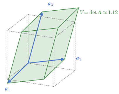
A \(3\times 3\) matrix \(\bm A = [\bm a_1\ \bm a_2\ \bm a_3]\) carries the unit cube to the parallelepiped spanned by its columns, Figure 3.11.2. Its signed volume is the scalar triple product of Chapter 3.7, which is the determinant with the three vectors as columns,
\[
\det\bm A = \bm a_1\cdot(\bm a_2\times\bm a_3)
\]
The plane reading carries over with volumes in place of areas. The map multiplies every volume by \(|\det\bm A|\). A negative determinant means that the columns form a left-handed system, and the map turns space inside out as a mirror does. A zero determinant means that the three columns lie in one plane, so that all of space collapses onto a plane, a line or a point.
Figure 3.11.2: The unit cube (dashed) and its image under a \(3\times 3\) matrix \(\bm A\), the parallelepiped spanned by the columns \(\bm a_1\), \(\bm a_2\), \(\bm a_3\). Its volume is \(\det\bm A\).
Cofactor expansion
Beyond three dimensions there is no picture to read, and the determinant of an \(n\times n\) matrix is defined by reducing it, step by step, to determinants of order \(2\). We pick a row \(i\). For each entry \(a_{ij}\) of that row we strike out row \(i\) and column \(j\); the determinant of the \((n-1)\times(n-1)\) matrix that remains is the minor\(M_{ij}\), and with a sign attached it is the cofactor
\[
C_{ij} = (-1)^{i+j}M_{ij}
\]
The determinant is the sum of the entries of the row times their cofactors,
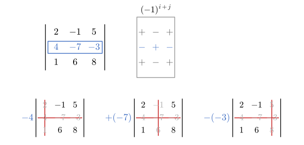
and expanding along a column \(j\) instead, \(\det\bm A = a_{1j}C_{1j} + \dots + a_{nj}C_{nj}\), gives the same value for every choice. For \(n > 3\) each minor is expanded in turn, until only determinants of order \(2\) remain. The factor \((-1)^{i+j}\) is \(+1\) or \(-1\) in a checkerboard pattern that starts with \(+\) in the top left corner,
Each zero entry removes a whole term from 3.11.2, so we expand along the row or column with the most zeros. Expanding a \(3\times 3\) determinant along its first column gives back the triple product \(u_1(v_2w_3 - v_3w_2) + u_2(v_3w_1 - v_1w_3) + u_3(v_1w_2 - v_2w_1)\) of Chapter 3.7. Many texts write the determinant with vertical bars, \(|\bm A| = \det\bm A\), as we do for the minors below.
Example 2: A determinant of order three
Figure 3.11.3: The matrix of Examples 2 and 3 with row 2 picked for the expansion, the checkerboard of signs, and the three minors of row 2, each with its row and column struck out.
The volume factor is \(114\), and it is positive, so the columns of \(\bm A\) form a right-handed system.
Practise the expansion of a determinant of order three below. The parallelepiped of the columns takes the colour of the sign of its volume once the answer is right.
The cost of the expansion
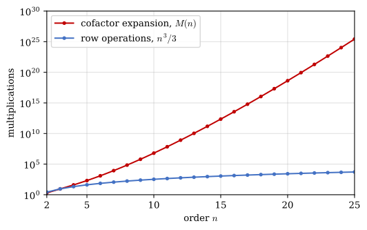
Cofactor expansion is a definition, and as a method of computation it does not scale. A determinant of order \(n\) needs \(n\) determinants of order \(n - 1\) and \(n\) multiplications by the entries of the row, so the number of multiplications obeys
which grows like \((e - 1)\,n!\). For \(n = 25\) this is about \(2.7\cdot 10^{25}\) multiplications. At a million multiplications per second they take \(2.7\cdot 10^{19}\) s, some sixty times the age of the universe, \(13.8\cdot 10^9\) years \(\approx 4.4\cdot 10^{17}\) s. Even at ten billion per second the wait is more than eighty million years. The row operations of Example 3 bring the matrix to triangular form with about \(n^3/3\) multiplications, some \(5\,200\) for \(n = 25\), which a computer finishes in microseconds.
Code
n = np.arange(2, 26)M = [2]for k in n[1:]: M.append(int(k)*(M[-1] +1)) # n minors of order n - 1, each times one entryM = np.array(M, dtype=float)age =13.8e9*365.25*24*3600# the age of the universe in secondsyears = M[-1]/1e6/(365.25*24*3600) # n = 25 at a million multiplications per second
For \(n = 25\) the count and the waiting time at a million multiplications per second are
\[ \begin{aligned}M(25) &\approx 2.67 \cdot 10^{25}\\ t &\approx 2.67 \cdot 10^{19}\text{ s} \approx 61.2\text{ ages of the universe}\end{aligned} \]
Figure 3.11.4 compares the two counts on a logarithmic scale.
Figure 3.11.4: The number of multiplications needed for a determinant of order \(n\). The expansion grows like \(n!\), the row operations like \(n^3\).
Rules for determinants
For square matrices \(\bm A\) and \(\bm B\) of order \(n\) and a number \(s\), the determinant obeys the rules
\[
\begin{aligned}
\det\bm A^\mathsf{T} &= \det\bm A && \text{transpose} \\
\det(\bm A\bm B) &= \det\bm A\,\det\bm B && \text{product} \\
\det(s\bm A) &= s^n\det\bm A && \text{scalar multiple} \\
\det\bm I &= 1 && \text{identity}
\end{aligned}
\tag{3.11.3}\]
and for the rows of \(\bm A\):
multiplying one row by \(s\) multiplies the determinant by \(s\);
adding a multiple of one row to another leaves the determinant unchanged;
swapping two rows changes the sign of the determinant;
two equal rows give the determinant zero.
By the first rule of 3.11.3 the same four rules hold for the columns, and for columns we see them in the picture. A column multiplied by \(s\) stretches one side of the parallelogram by \(s\), and its area follows. Adding a multiple of \(\bm a_1\) to \(\bm a_2\) slides the tip of \(\bm a_2\) parallel to \(\bm a_1\), a shear that keeps the base and the height. Swapping the columns reverses the turn from the first to the second, and two equal columns span no area at all.
Multiplying the whole matrix by \(s\) stretches all \(n\) columns, so the volume grows by \(s^n\), not by \(s\). The determinant of a sum is in general no sum of determinants, \(\det(\bm A + \bm B)\neq\det\bm A + \det\bm B\).
The product rule says that areas scale twice. The product \(\bm A\bm B\) is the map \(\bm B\) followed by the map \(\bm A\) (Chapter 3.10): \(\bm B\) multiplies every area by \(\det\bm B\), then \(\bm A\) multiplies the result by \(\det\bm A\). In the video \(\bm B\) has \(\det\bm B = 1.5\) and \(\bm A\) has \(\det\bm A = 2\), and the readout of the current matrix ends at \(3\).
For \(2\times 2\) matrices SymPy confirms the product rule with general entries: the difference of the two sides expands to zero.
A triangular matrix has zeros on one side of its diagonal. Expanding along its first column leaves one term, the first diagonal entry times the triangular minor below it, and repeating the step gives the product of the diagonal entries,
The row rules turn any square matrix into a triangular one, and they keep track of the determinant on the way: rule 2 leaves it alone, and each swap of rule 3 flips its sign. This is the fast route of Figure 3.11.4.
Example 3: A determinant by row operations
Compute the determinant of the matrix of Example 2, Figure 3.11.3, by bringing it to triangular form.
A \(1\) in the top left corner keeps the numbers simple, so we swap rows 1 and 3, which changes the sign. Subtracting \(4\) times the new row 1 from row 2 and \(2\) times it from row 3 leaves the determinant unchanged and clears the first column below the diagonal,
Subtracting \(\tfrac{13}{31}\) times row 2 from row 3 clears the last entry below the diagonal, \(-11 - \tfrac{13}{31}(-35) = \tfrac{114}{31}\), and 3.11.4 gives
The value \(114\) of Example 2 returns from three subtractions and one swap. AA.det() in SymPy and np.linalg.det(A) in NumPy compute determinants this way.
The inverse: the map undone
The map \(\bm x\mapsto\bm A\bm x\) carries each vector to its image. The inverse map carries each image back to where it came from. Its matrix is the inverse\(\bm A^{-1}\), defined by
The first product undoes \(\bm A\) after it has acted, the second does \(\bm A\) after \(\bm A^{-1}\) has acted, and both leave every vector where it was. A matrix that has an inverse is called invertible. Only a square matrix can have one, since both products must be defined and equal to the same \(\bm I\). Played on the plane, the map \(\bm A = \begin{bmatrix} 2 & 1\\ 1 & 1\end{bmatrix}\) carries the plane and the vector \(\bm u\) away, and applying \(\bm A^{-1} = \begin{bmatrix} 1 & -1\\ -1 & 2\end{bmatrix}\) after it brings everything back to the identity.
Grant Sanderson shows the same picture in the video below and asks what happens when the map flattens the plane. Its second half, on column space and null space, returns in Chapter 3.12.
A matrix has at most one inverse. Suppose that \(\bm B\) and \(\bm C\) both satisfy 3.11.5. Inserting \(\bm I = \bm A\bm B\) and regrouping the product gives
\[
\bm C = \bm C\bm I = \bm C(\bm A\bm B) = (\bm C\bm A)\bm B = \bm I\bm B = \bm B
\]
so the two are the same matrix, and we may speak of the inverse.
The determinant decides whether the inverse exists. Taking the determinant of 3.11.5 and using the product rule of 3.11.3 gives \(\det\bm A\,\det\bm A^{-1} = \det\bm I = 1\), so
\[
\det\bm A^{-1} = \frac{1}{\det\bm A}
\]
which is impossible when \(\det\bm A = 0\). A singular matrix has no inverse, as the collapse of the plane told us: two vectors with the same image cannot both be sent back. The inverse undoes the area factor: a map that enlarges areas five times has an inverse that shrinks them to a fifth.
and dividing by \(\det\bm A\) leaves \(\bm I\). The matrix in 3.11.6 holds the cofactors of \(\bm A\), transposed. That holds for every \(n\), \(\bm A^{-1} = \bm C^\mathsf{T}/\det\bm A\) with \(\bm C\) the matrix of cofactors \(C_{ij}\), the formula Cayley refers to in the quotation. With \(n\) cofactors of order \(n-1\) in every row, it inherits the cost of the expansion, so beyond \(n = 3\) we leave inverses to the computer.
Example 4: The inverse of a \(2\times 2\) matrix
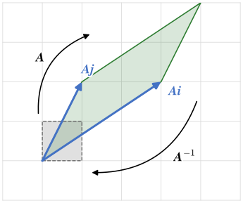
Figure 3.11.5: The map \(\bm A\) carries the unit square to the parallelogram of its columns \(\bm A\bm i\) and \(\bm A\bm j\), and \(\bm A^{-1}\) carries it back.
Find the inverse of \(\bm A = \begin{bmatrix} 3 & 1\\ 2 & 2\end{bmatrix}\), Figure 3.11.5, and check it.
The determinant is \(\det\bm A = 3\cdot 2 - 1\cdot 2 = 4\), so the inverse exists, and 3.11.6 gives
The determinant of the inverse is \(1/\det\bm A = 1/4\): the parallelogram of Figure 3.11.5 has four times the area of the square, and \(\bm A^{-1}\) shrinks it back.
The inverse of a larger matrix is computed the same way in code. For
Every entry has the denominator \(71\), the absolute value of the determinant, since \(\bm A^{-1} = \bm C^\mathsf{T}/\det\bm A\) divides the integer cofactors by \(\det\bm A = -71\).
Practise the \(2\times 2\) inverse below. Fractions such as 1/4 may be typed as they are. Once the answer is right, the images of \(\bm i\) and \(\bm j\) under \(\bm A^{-1}\) are drawn in green.
Rules for inverses
For invertible matrices \(\bm A\) and \(\bm B\) of the same order and a number \(s\neq 0\),
Each rule is checked by multiplying the claimed inverse with the matrix and finding \(\bm I\). For the product,
\[
(\bm B^{-1}\bm A^{-1})(\bm A\bm B) = \bm B^{-1}(\bm A^{-1}\bm A)\bm B = \bm B^{-1}\bm I\bm B = \bm B^{-1}\bm B = \bm I
\]
The order reverses. The map \(\bm A\bm B\) applies \(\bm B\) first and \(\bm A\) second, so undoing it removes \(\bm A\) first and \(\bm B\) second, as we take off the shoes before the socks. For the transpose, \((\bm A^{-1})^\mathsf{T}\bm A^\mathsf{T} = (\bm A\bm A^{-1})^\mathsf{T} = \bm I^\mathsf{T} = \bm I\) by the transpose rule of Chapter 3.10.
Example 5: A matrix equation
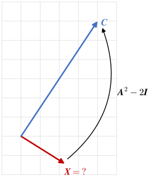
Figure 3.11.6: The map \(\bm A^2 - 2\bm I\) carries the unknown \(\bm X\) to the known column \(\bm C\).
Solve \(\bm A^2\bm X = 2\bm X + \bm C\) for the column \(\bm X\), with
\[
\bm A = \begin{bmatrix} 2 & 1\\ 1 & 0\end{bmatrix}, \qquad \bm C = \begin{bmatrix} 4\\ 6\end{bmatrix}
\]
We collect the terms with \(\bm X\) on the left. Factoring \(\bm X\) out of \(\bm A^2\bm X - 2\bm X\) needs the identity: the bracket \((\bm A^2 - 2)\) would subtract a number from a matrix, so we write \(2\bm X = 2\bm I\bm X\) first,
\[
\bm A^2\bm X - 2\bm I\bm X = \bm C
\quad\Longleftrightarrow\quad
(\bm A^2 - 2\bm I)\bm X = \bm C
\quad\Longleftrightarrow\quad
\bm X = (\bm A^2 - 2\bm I)^{-1}\bm C
\]
The inverse multiplies \(\bm C\) from the left, as it multiplied \(\bm X\) from the left; \(\bm C(\bm A^2 - 2\bm I)^{-1}\) would not even have matching sizes. The matrix \(\bm A^2 - 2\bm I\) is the map that carries \(\bm X\) to \(\bm C\) in Figure 3.11.6, and with 3.11.6
and the check inserts \(\bm X\) in the original equation.
Code
AA = sp.Matrix([[2, 1], [1, 0]])CC = sp.Matrix([4, 6])NN = AA**2-2*sp.eye(2) # sp.eye(2) is the identity that the factoring needsXX = NN.inv()*CCcheck = AA**2*XX - (2*XX + CC)
The solution and the check are
\[ \bm X = \left[\begin{matrix}\dfrac{16}{7}\\- \dfrac{10}{7}\end{matrix}\right],\qquad \bm A^2\bm X - (2\bm X + \bm C) = \left[\begin{matrix}0\\0\end{matrix}\right] \]
Both sides of the equation agree at \([60/7,\ 22/7]^\mathsf{T}\).
Practise matrix equations of the same type below.
WarningNever invert a matrix to solve a system
The solution \(\bm X = (\bm A^2 - 2\bm I)^{-1}\bm C\) is right on paper, and in a \(2\times 2\) exercise the inverse is the quickest way there. On a computer we do not form the inverse to solve \(\bm A\bm x = \bm b\). Computing \(\bm A^{-1}\) takes about three times as many operations as solving the system directly by elimination; it collects more round-off error on the way; and when \(\bm A\) is nearly singular, the inverse magnifies that error further. The large matrices of mechanics are also mostly zeros, and their inverses are not. We write np.linalg.solve(A, b) or sp.Matrix.LUsolve instead, as Chapter 3.12 shows.
is called orthogonal. Its inverse costs nothing, \(\bm Q^{-1} = \bm Q^\mathsf{T}\). The entry \((i, j)\) of \(\bm Q^\mathsf{T}\bm Q\) is row \(i\) of \(\bm Q^\mathsf{T}\) times column \(j\) of \(\bm Q\), which is \(\bm q_i^\mathsf{T}\bm q_j\), the dot product of columns \(i\) and \(j\) (Chapter 3.6). The identity has ones on its diagonal and zeros elsewhere, so 3.11.8 says that every column has unit length and that any two columns are perpendicular: the columns of an orthogonal matrix are orthonormal.
An orthogonal map keeps dot products, and with them lengths and angles. For any vectors \(\bm a\) and \(\bm b\),
\[
(\bm Q\bm a)^\mathsf{T}(\bm Q\bm b) = \bm a^\mathsf{T}\bm Q^\mathsf{T}\bm Q\,\bm b = \bm a^\mathsf{T}\bm b
\]
so \(|\bm Q\bm a| = |\bm a|\), and perpendicular vectors stay perpendicular. The determinant follows from 3.11.3, \(\det(\bm Q^\mathsf{T}\bm Q) = (\det\bm Q)^2 = \det\bm I = 1\), so \(\det\bm Q = \pm 1\): an orthogonal map keeps areas. With \(\det\bm Q = 1\) it is a rotation, with \(\det\bm Q = -1\) a reflection, which turns the plane over. The product of two orthogonal matrices is orthogonal, since \((\bm P\bm Q)^\mathsf{T}\bm P\bm Q = \bm Q^\mathsf{T}\bm P^\mathsf{T}\bm P\bm Q = \bm Q^\mathsf{T}\bm Q = \bm I\), and so are \(\bm Q^\mathsf{T}\) and \(\bm I\).
Example 6: The plane rotation
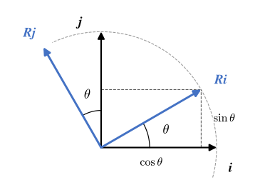
Figure 3.11.7: The rotation \(\bm R\) turns \(\bm i\) and \(\bm j\) through the angle \(\theta\). The images \(\bm R\bm i\) and \(\bm R\bm j\) are the columns of \(\bm R\).
The rotation of the plane through the angle \(\theta\) turns \(\bm i\) to \([\cos\theta,\ \sin\theta]^\mathsf{T}\) and \(\bm j\) to \([-\sin\theta,\ \cos\theta]^\mathsf{T}\), Figure 3.11.7. Write its matrix \(\bm R\), show that it is orthogonal with \(\det\bm R = 1\), and find \(\bm R^{-1}\) for \(\theta = 30^\circ\).
The images of \(\bm i\) and \(\bm j\) are the columns,
Each column has the length \(\sqrt{\cos^2\theta + \sin^2\theta} = 1\), and their dot product \(-\cos\theta\sin\theta + \sin\theta\cos\theta\) vanishes, so \(\bm R^\mathsf{T}\bm R = \bm I\). The determinant is \(\cos^2\theta + \sin^2\theta = 1\). The inverse is the transpose,
RR.inv() computes what the transpose gives for free. The last video turns the plane through \(30^\circ\): the square stays a unit square, \(\det\bm R\) stays \(1\) and the length of \(\bm u\) does not change. The transpose then turns everything back. Chapter 3.13 derives \(\bm R\) from the sum formulas and extends it to rotations in space.
Practise orthogonal matrices below. Some are rotations and some are reflections; the determinant tells which.