The draw latchsv. spännlås on a toolbox snaps shut and stays shut. Pull on the lid as hard as you like and the latch only presses harder into its closed position, yet a light flick of the lever opens it. The same thing happens in locking pliers, in the toggle clampsv. snabbspännare that holds a workpiece on a drilling table, in a wall switch that clicks between on and off, and in the brace of a folding table leg. Each of these devices has three pivots. Two of the distances between them are fixed by rigid parts, the third changes as the device moves, and the device works because it is parked just past the position where the three pivots lie on one line. That position is the dead centresv. dödläge, and a mechanism built to rest slightly beyond it is an over-centre mechanism.
Figure 11.5.1: Michael Laws of Teaching Tech designs and prints four over-centre mechanisms: a lever with a rubber band (from 1:00), a draw latch (3:07), two snap latches that work by compression (5:38) and the trigger of a CO2 dragster launcher (8:22) [1].
Figure 11.5.1 is a good place to start, because every device in it can be printed and handled. The video summarises the rule as three pivots, two fixed distances and one variable one, with the peak resistance where the three line up. In this chapter we turn that rule into mechanics. We set up the geometry of the three pivots and find the moment a stretched member exerts about the pivot, which vanishes at the dead centre and changes sign across it. Virtual work then gives the force amplification near the dead centre, the reason a knee joint or a punch press can produce forces far larger than the effort. The potential energy of the elastic member explains the snap, and the stop explains why the closed position holds any load the parts can carry. A toggle clamp is then analysed by hand and checked in a motion solver, the Python counterpart of SolidWorks Motion. The chapter ends with the cargo door of Turkish Airlines Flight 981, whose latches never reached their dead centre.
Three pivots and one varying length
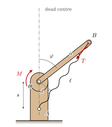
Figure 11.5.2 shows the simplest over-centre mechanism, the first one of Figure 11.5.1. A lever \(OB\) of length \(a\) turns about the pivot \(O\) on a base. The base also carries the anchor \(A\), a distance \(s\) from \(O\), and an elastic member, here a rubber band, connects \(A\) to the lever’s end \(B\). The distances \(a\) and \(s\) are fixed by the two rigid parts. The length \(\ell = |AB|\) of the band is the variable one.
Figure 11.5.2: The three pivots. The lever \(OB\) turns about \(O\); the band \(AB\) pulls \(B\) towards the anchor \(A\) with the tension \(T\). The angle \(\varphi\) is measured at \(O\) from the dead centre line, the extension of \(AO\) beyond \(O\), and \(d\) is the lever arm of the band about \(O\). \(M\) is the moment of the band on the lever, positive in the sense of increasing \(\varphi\).
We measure the lever’s angle \(\varphi\) from the line through \(A\) and \(O\), extended beyond \(O\). The angle between \(OA\) and \(OB\) is then \(\pi - \varphi\), and the law of cosines in the triangle \(OAB\) gives the length of the band,
The length is largest, \(\ell = a + s\), at \(\varphi = 0\), where \(A\), \(O\) and \(B\) lie on one line with \(O\) in the middle, and it falls symmetrically on both sides. For Teaching Tech’s lever, \(a = 45\) mm and \(s = 12\) mm, the band is 57 mm long when the lever points straight up and about 44 mm when the lever lies on the base, the numbers read off the sketch in the video.
The band pulls \(B\) towards \(A\) with its tension \(T\). The moment of this force about \(O\) follows from virtual work without a free body diagram. When the lever turns by \(\delta\varphi\) the band lengthens by \(\delta\ell\), and the band’s force does the work \(-T\,\delta\ell\) on the lever, negative because the force opposes the lengthening. The same work, written with the moment \(M\) of the band about \(O\), is \(M\,\delta\varphi\). Setting the two equal gives
\[
M = -T\,\frac{d\ell}{d\varphi}
\tag{11.5.2}\]
the rule of Virtual work: a force times the derivative of the length it acts along. Differentiating 11.5.1 gives the derivative of the length.
Code
a, s, T, phi = sp.symbols('a, s, T, varphi', positive=True)ell = sp.sqrt(a**2+ s**2+2*a*s*sp.cos(phi)) # @eq-oc-lengthdell = sp.diff(ell, phi)M_band = sp.simplify(-T*dell) # @eq-oc-moment-vw# the same moment as T times the lever arm d: twice the area of OAB is a s sin(phi) = ell dd_arm = a*s*sp.sin(phi)/ellcheck = sp.simplify(M_band - T*d_arm)
The derivative and the moment are
\[ \begin{aligned}\frac{d\ell}{d\varphi} &=- \dfrac{a s \sin{\left(\varphi \right)}}{\sqrt{a^{2} + 2 a s \cos{\left(\varphi \right)} + s^{2}}}\\ M &=\dfrac{T a s \sin{\left(\varphi \right)}}{\sqrt{a^{2} + 2 a s \cos{\left(\varphi \right)} + s^{2}}}\end{aligned} \]
The same result comes from the lever arm. Twice the area of the triangle \(OAB\) is \(as\sin\varphi\), from the two sides at \(O\), and it is also \(\ell d\), from the side \(AB\) and its height \(d\) over \(O\). So \(d = as\sin\varphi/\ell\) and \(M = Td\), which the code above confirms (check is zero):
\[
M = T d = \frac{T a s \sin\varphi}{\ell}
\tag{11.5.3}\]
11.5.3 holds the whole over-centre idea. The moment is zero at \(\varphi = 0\), however large the tension, because the line of the band then passes through the pivot. It is positive for \(\varphi > 0\) and negative for \(\varphi < 0\): on either side of the dead centre the band turns the lever away from it. A lever placed at \(\varphi = 0\) is in equilibrium, but the slightest disturbance sends it to one side or the other, which is Teaching Tech’s observation that the mechanism “wants to be anywhere except perfectly vertical over-centre”.
Read backwards, 11.5.3 is a force amplifier. A moment \(M\) on the lever, resisted by the member \(AB\), produces the force
\[
T = \frac{M\ell}{as\sin\varphi}
\]
which grows without bound as \(\varphi \to 0\). Near the dead centre a small effort on the lever is balanced by an enormous force in the member. The ratio of output to input force is the mechanical advantagesv. kraftutväxling of the mechanism, and the next example is the classic device built on it.
Example 1: The knee toggle
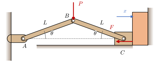
Two links of equal length \(L\) form a knee (Figure 11.5.3). The link \(AB\) turns about the fixed pin \(A\), the link \(BC\) connects the knee \(B\) to a slider \(C\) that runs on a horizontal guide and presses a workpiece. Both links make the angle \(\theta\) with the line \(AC\). A force \(P\) pushes the knee straight down. Find the force \(F\) with which the slider presses the workpiece, as a function of \(\theta\), and its value for \(P = 100\) N at \(\theta = 10°\), \(2°\) and \(0.5°\). Friction and the weight of the links are neglected.
Figure 11.5.3: The knee toggle of Example 1. \(P\) pushes the knee \(B\) down; the workpiece pushes back on the slider with \(F\). Both links make the angle \(\theta\) with \(AC\), and the slider moves along \(x\).
The mechanism has one degree of freedom, \(\theta\), and the pins and the guide do no virtual work, so we use virtual work directly. With \(A\) at the origin the knee is at height \(y_B = L\sin\theta\) and the slider at \(x_C = 2L\cos\theta\). The force \(P\) points down, the workpiece force \(F\) points in \(-x\), and the virtual work of the two is
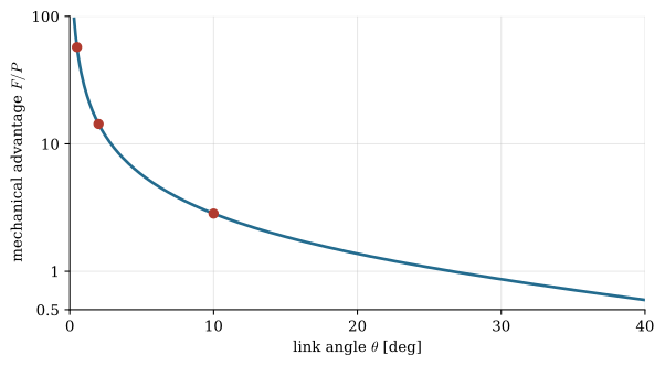
Figure 11.5.4: The mechanical advantage \(F/P = 1/(2\tan\theta)\) of the knee toggle. The points are the three angles of Example 1.
The force on the workpiece is 2.8 times the push at \(\theta = 10°\), 14 times at \(2°\) and 57 times at half a degree (Figure 11.5.4), and 11.5.2 tells us why: the slider barely moves when the knee is almost straight, so a small force on the knee does the same work as a large force on the slider. Stone crushers, riveting presses and coin minting presses use this, and so does a person standing with straight knees: the muscles hold almost nothing while the leg bones carry the weight through the dead centre.
The formula also says \(F \to \infty\) at \(\theta = 0\), which no press delivers. It assumes rigid links and a rigid workpiece, so the slider cannot move once it touches. Real parts deform, and the elastic deformation sets the force. That is the subject of the next section.
Energy: why the mechanism snaps
Let the member \(AB\) be elastic, with stiffness \(k\) and free length \(\ell_0\). A rubber band, a spring or a printed part that stretches a little all fit this model as long as the member is in tension, \(\ell > \ell_0\). Its potential energy is
and the moment it exerts on the lever is \(M = -dU/d\varphi = -k(\ell - \ell_0)\,d\ell/d\varphi\), which is 11.5.2 with \(T = k(\ell - \ell_0)\). The lever is in equilibrium wherever \(dU/d\varphi = 0\), and as shown in Potential energy and stability the equilibrium is stable where \(U\) has a minimum and unstable where it has a maximum. At the dead centre \(d\ell/d\varphi = 0\), so \(\varphi = 0\) is always an equilibrium. Its stability follows from the second derivative.
Evaluated at the dead centre, the second derivative is
\[ \left.\frac{d^2U}{d\varphi^2}\right|_{\varphi=0} =\dfrac{a k s \left(\ell_{0} - \sqrt{a^{2} + 2 a s + s^{2}}\right)}{a + s} \]
which is negative whenever the member is stretched at the dead centre, \(\ell_0 < a + s\). The dead centre is then a maximum of the energy, an unstable equilibrium, with the energy falling on both sides. The member’s own minimum would lie where \(\ell = \ell_0\), far down on either side, and something has to stop the lever before it gets there. In the toolbox latch it is the lid or the base, in Teaching Tech’s lever it is the base plate. The lever comes to rest against this stop with the member still stretched, and the moment of 11.5.3 presses it into the stop.
So an over-centre mechanism has two states. In each of them the lever lies against a stop on its own side of the dead centre, and between them lies an energy barrier, the difference between \(U(0)\) and the energy at the stop. To change state, we must supply that energy, and once the lever is past the top of the barrier, the member releases it again and the lever snaps to the other stop. Teaching Tech’s dragster launcher stores the energy of a strong spring in this way and releases it with a nudge from a small solenoid.
Example 2: The rubber band lever
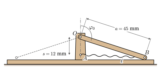
The lever of Figure 11.5.1, drawn to scale in Figure 11.5.5, has \(a = 45\) mm and \(s = 12\) mm. It rests on the base plate at \(\varphi_0 = \pm 108°\). A rubber band with free length \(\ell_0 = 30\) mm and stiffness \(k = 0.15\) N/mm, assumed values for a small office band that we take as linear, connects \(A\) and \(B\). Find the band tension and the moment that hold the lever on the plate, the energy needed to flip it to the other side, and the largest moment the finger must apply on the way.
Figure 11.5.5: The rubber band lever of Example 2, to scale. The lever rests on the plate at \(\varphi_0 = 108°\); the dashed line marks the other rest position, at \(-108°\). The band is drawn as a coil.
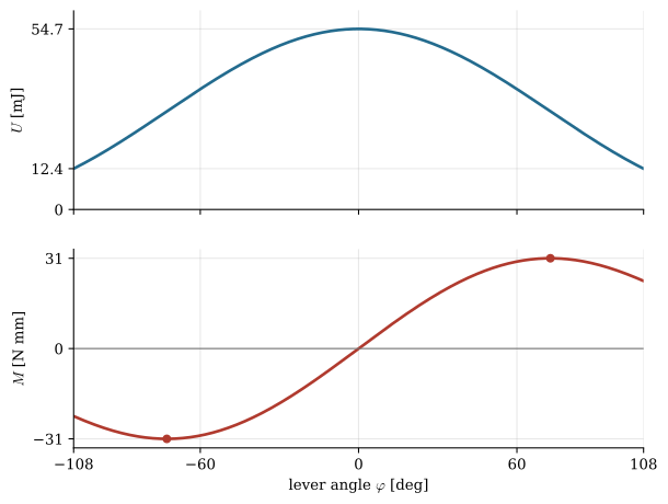
We evaluate 11.5.1, 11.5.3 and 11.5.4 over the range between the two stops, and check the energy against the work of the moment: integrating \(M\) from the dead centre to the stop must give the energy released, \(U(0) - U(\varphi_0)\).
Code
a_b, s_b, k_b, l0_b =45.0, 12.0, 0.15, 30.0# [mm], [mm], [N/mm], [mm]phi_0 = np.radians(108.0) # the stopell_f = sp.lambdify((a, s, phi), ell)phis = np.linspace(-phi_0, phi_0, 2001)ell_b = ell_f(a_b, s_b, phis)T_b = k_b*np.maximum(ell_b - l0_b, 0) # a band carries no compression [N]M_b = T_b*a_b*s_b*np.sin(phis)/ell_b # @eq-oc-moment [N mm]U_b =0.5*k_b*np.maximum(ell_b - l0_b, 0)**2# @eq-oc-energy [N mm]i0 =len(phis)//2# the dead centre, phi = 0T_stop, M_stop = T_b[-1], M_b[-1]dU = U_b[i0] - U_b[-1] # the barrier, in N mm = mJW_M = np.trapezoid(M_b[i0:], phis[i0:]) # work of M from the centre to the stopi_pk = i0 + np.argmax(M_b[i0:])M_peak, phi_peak = M_b[i_pk], np.degrees(phis[i_pk])
With these values the lever is held on the plate by
Figure 11.5.6: The energy of the band (top) and its moment on the lever (bottom) between the two stops of Example 2. The dead centre at \(\varphi = 0\) is the top of the barrier; the moment peaks at the dots and is zero at the dead centre.
The lever lies on the plate with a band tension of about 2 N, and the band presses it down with the moment \(M(\varphi_0)\). Flipping it costs the barrier energy of about 42 mJ, and the integral of the moment returns the same energy, which checks 11.5.3 against 11.5.4. The lower panel of Figure 11.5.6 refines the statement of the video that the resistance increases towards the centre. The tension does, it is largest at the dead centre. The moment the finger has to overcome peaks well before it, at about \(\pm 73°\), and then falls to zero, because the lever arm \(d\) shrinks faster than the tension grows. Near the top the lever balances on a knife edge, and a breath tips it.
Example 3: A latch without a spring
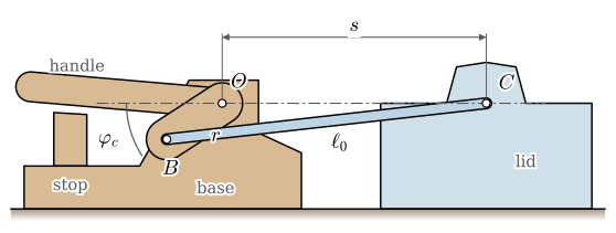
The draw latch of Figure 11.5.1 (from 3:07 in the video) has no rubber band. Its handle turns about the pivot \(O\) on the base and carries the pin \(B\) a distance \(r\) from \(O\) (Figure 11.5.7). A rigid printed bail of length \(\ell_0\) runs from \(B\) to the keeper \(C\) on the lid, a distance \(s\) from \(O\). Closed, the handle lies on its stop with \(B\) past the line \(OC\) by the angle \(\varphi_c\), and the bail is unstrained. To go from open to closed, \(B\) must pass the dead centre, where the distance \(|BC| = r + s\) is longer than the bail. The bail has to stretch by
\[
\delta = r + s - \ell_0
\]
and the latch only works because the printed material allows it. From the sketch in the video, \(s \approx 40\) mm and \(r \approx 5.6\) mm, and the closed bail measures \(\ell_0 = 44.83\) mm; the video reports the difference as an arm length delta of 0.822 mm. Find the strain the bail must take, and how it depends on \(r\) and \(\varphi_c\). A second, exaggerated version in the video has a bail of about 54 mm and a delta of 1.45 mm.
Figure 11.5.7: The draw latch of Example 3, closed, with the handle on its stop and the pin \(B\) past the line \(OC\) by \(\varphi_c\). The radius \(r\) is drawn about twice its size.
The dead centre is the position with \(B\) on the line \(OC\), beyond \(O\). The bail is relaxed when closed, so 11.5.1 with \(a = r\) and \(\varphi = \varphi_c\) gives its length, \(\ell_0^2 = r^2 + s^2 + 2rs\cos\varphi_c\). Subtracting this from \((r+s)^2\) gives the stretch at the dead centre exactly,
where the approximation uses \(1 - \cos\varphi_c \approx \varphi_c^2/2\) and \(\ell_0 \approx r + s\).
Code
r_l, s_l, dl_v =5.6, 40.0, 0.822# [mm], from the video's sketchl0_l =44.83# the closed bail [mm]eps_l = dl_v/l0_l # the strain at the dead centreeps_big =1.45/54.0# the exaggerated version# the closing angle that the video's numbers imply, from the exact @eq-oc-stretchphi_c = np.degrees(np.arccos(1- dl_v*(r_l + s_l + l0_l)/(2*r_l*s_l)))
The strain in the bail as it passes the dead centre, and the closing angle that the video’s numbers imply, are
A strain of 1.8 % is not small for a printed polymer. The printed PLA of the tensile test reaches its maximum stress near 2 % strain, so a PLA bail is taken to the edge of its strength each time the latch closes and opens, and the exaggerated version at 2.7 % goes beyond it. This is what Teaching Tech felt, a PLA latch that works but “feels like it’s going to break”, and why the video recommends PETG, which yields and stretches further before it fails. In practice the strain is smaller than this estimate, because the pin clearances and the bending of the handle and the bail take part of \(\delta\), and in a printed part the clearances are not small.
11.5.5 is the design rule behind the video’s second piece of advice, to keep the two closest pivots close together. For \(r \ll s\) the stretch is about \(r\varphi_c^2/2\), proportional to \(r\) and to the square of the closing angle. Halving \(r\) halves the strain; halving \(\varphi_c\) quarters it. The angle cannot be made very small, though, as the next section shows. A latch that is also meant to pull the lid tight, against a seal for example, is made with a bail slightly shorter than the closed distance \(|BC|\), so that a preload \(k\,(|BC| - \ell_0)\) remains in the closed position.
The stop, and what holds the load
In the closed position the lever rests on its stop at \(\varphi_s > 0\), and a load on the closed device, the lid pushed open or the workpiece pushing back, adds tension to the member. By 11.5.3 that tension turns the lever further into the stop, with the small lever arm
so the moment on the stop is only \(Td_s\), the load times a lever arm of a few millimetres, and the mechanism holds as long as its parts are strong enough. Friction plays no part, unlike in a screw or a wedge, which are held by friction and loosened by vibration.
Two things can undo this. The first is a lever that never reaches its stop: with \(\varphi_s < 0\) the load turns the lever away from the stop, back towards the open position, and whatever drives the lever has to hold it. The second is a lever that does reach the stop but with \(d_s\) so small that it is consumed by the play in the pins and by the elastic deflection of the parts under load. The line of the force then moves back across the pivot and the mechanism reverses. The offset \(d_s\) must therefore be larger than the sum of the pin clearances and deflections in the load path. This sets a lower bound on \(\varphi_s\) that competes with 11.5.5, which favours a small angle. For the latch of Example 3, \(d_s = rs\sin\varphi_c/\ell_0 = 2.8\) mm, ample for printed pins with a few tenths of a millimetre of play.
Example 4: A toggle clamp in a motion solver
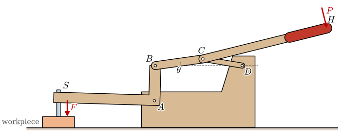
The horizontal toggle clamp of Figure 11.5.8 is a four-bar linkage. The arm turns about \(A\) on the base and carries the spindle \(S\) at the distance \(|AS| = 60\) mm. The handle is pinned to the arm at \(B\), with \(|AB| = 22\) mm, and a short link \(CD\) connects the handle at \(C\) to the base at \(D\), with \(|BC| = 30\) mm and \(|CD| = 25\) mm. The grip \(H\) is 80 mm beyond \(C\), the handle being bent upwards by \(6°\) at \(C\) so that it clears the pin \(D\). The pin \(D\) is placed so that the dead centre comes with the arm upright: \(D\) lies 55 mm to the right of \(A\) and 22 mm above it. The handle angle \(\theta\) is measured at \(B\) from the horizontal. The spindle touches the workpiece at \(\theta_c = 10°\), and from there the workpiece and the rubber tip of the spindle act as a spring of stiffness \(k = 200\) N/mm. The handle closes against a stop at \(\theta_s = -3°\). Find the clamping force \(F\), the moment \(M\) and the hand force \(P\) at \(H\), perpendicular to the handle, as the handle closes from \(\theta_c\) to the stop, and check the hand solution with a motion solver.
Figure 11.5.8: The horizontal toggle clamp of Example 4, at \(\theta = 8°\) on its way to the dead centre. The arm turns about \(A\), the handle about \(B\) on the arm, the link \(CD\) about \(D\) on the base. The workpiece pushes the spindle up with the clamping force; \(F\) is drawn as the force of the spindle on the workpiece.
Step 1: The hand solution by virtual work
The loop \(A\), \(B\), \(C\), \(D\) gives the arm angle \(\alpha\) (of \(AB\)) as a function of the handle angle \(\theta\): \(C = A + b\,\bm e(\alpha) + c\,\bm e(\theta)\) must lie the distance \(e\) from \(D\), with \(\bm e(\psi) = (\cos\psi, \sin\psi)\) and \(b\), \(c\), \(e\) the lengths of \(AB\), \(BC\) and \(CD\). This is one equation for \(\alpha\), solved numerically on the branch where the arm stands upright. The spindle is at the height \(y_S = |AS|\cos\alpha\), the clamping force is \(F = k\,(y_S(\theta_c) - y_S(\theta))\), and virtual work with the pins doing no work gives the moment that must act on the handle,
and the hand force from \(P\,\bm n \cdot \delta\bm r_H = M\,\delta\theta\), with \(\bm n\) the unit normal to the handle \(CH\). The derivatives are taken by central differences of the loop solution.
Code
b_c, c_c, e_c, g_c, Ls_c =22.0, 30.0, 25.0, 80.0, 60.0# |AB|, |BC|, |CD|, |CH|, |AS| [mm]crank = np.radians(6.0) # the bend of the handle at Ck_c =200.0# workpiece and spindle tip [N/mm]th_c, th_s = np.radians(10.0), np.radians(-3.0) # contact and stopA_c, D_c = np.array([0.0, 0.0]), np.array([c_c + e_c, b_c])ee =lambda psi: np.array([np.cos(psi), np.sin(psi)])def alpha_of(theta):"""Arm angle for the handle angle theta, on the branch with the arm upright."""ifabs(theta) <1e-12:return np.pi/2# the dead centre, by construction gap =lambda al: np.linalg.norm(A_c + b_c*ee(al) + c_c*ee(theta) - D_c) - e_creturn brentq(gap, np.pi/2-0.8, np.pi/2)y_S =lambda theta: Ls_c*np.cos(alpha_of(theta))r_H =lambda theta: A_c + b_c*ee(alpha_of(theta)) + c_c*ee(theta) + g_c*ee(theta + crank)h =1e-7# step for the central differencesthetas = np.radians(np.linspace(10.0, -3.0, 521))F_c = np.array([k_c*(y_S(th_c) - y_S(t)) for t in thetas]) # [N]dyS = np.array([(y_S(t + h) - y_S(t - h))/(2*h) for t in thetas]) # [mm/rad]M_c =-F_c*dyS/1000# [N m]drH = np.array([(r_H(t + h) - r_H(t - h))/(2*h) for t in thetas]) # [mm/rad]n_H = np.array([[-np.sin(t + crank), np.cos(t + crank)] for t in thetas]) # normal to CHP_c =-M_c*1000/np.einsum('ij,ij->i', n_H, drH) # [N], positive pushing the grip downi_dc = np.argmin(np.abs(thetas))i_P = np.argmax(P_c)F_max, F_stop, P_max, th_Pmax, P_stop = F_c.max(), F_c[-1], P_c[i_P], np.degrees(thetas[i_P]), P_c[-1]
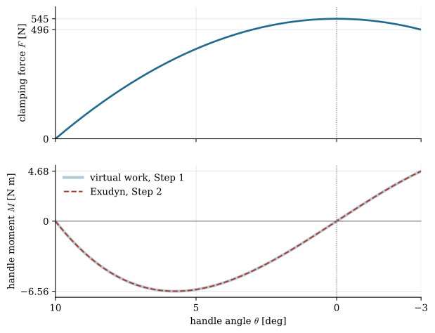
The clamping force is largest at the dead centre and slightly smaller at the stop; the hand force peaks on the way:
The hand force at the stop is negative: the handle no longer needs to be pushed, it is pulled into the stop by the clamp, and the stop takes over the role of the hand.
Step 2: The same clamp in a motion solver
SolidWorks Motion builds the same model from the assembly: rigid bodies with mass, ideal joints, a spring for the workpiece and a rotary motor that drives the handle, and it reports the motor torque and the joint forces. In Python, a solver of the same kind is Exudyn [2]. It describes each body by the coordinates of a reference frame and each joint by constraint equations, and solves for the motion and the Lagrange multipliers of the constraints, the method of How a motion solver works. The closed loop of the four-bar needs no special treatment. We give the three moving bodies small masses, prescribe the handle angle with a coordinate constraint that turns it from \(10°\) to \(-3°\) in 4 s, starting and stopping without a jump in speed and slow enough for inertia to be negligible, and read the moment from the multiplier of that constraint. The workpiece is a Cartesian spring at \(S\), stiff in \(y\) only. The other Python solvers, and the reasons for this one, are compared in Simulating mechanisms in Python.
Code
import exudyn as exufrom exudyn.itemInterface import (ObjectGround, NodePointGround, NodeRigidBody2D, ObjectRigidBody2D, MarkerBodyPosition, MarkerNodeCoordinate, RevoluteJoint2D, CartesianSpringDamper, CoordinateConstraint, SensorObject, SensorNode)mm =1e-3SC = exu.SystemContainer()mbs = SC.AddSystem()ground = mbs.AddObject(ObjectGround())n_gnd = mbs.AddNode(NodePointGround())def rigid_body(position, angle, mass, inertia):"""A planar rigid body with its reference point at a pin.""" node = mbs.AddNode(NodeRigidBody2D(referenceCoordinates=[*position, angle]))return mbs.AddObject(ObjectRigidBody2D(physicsMass=mass, physicsInertia=inertia, nodeNumber=node)), nodedef marker(body, local):return mbs.AddMarker(MarkerBodyPosition(bodyNumber=body, localPosition=[*local, 0.0]))al0 = alpha_of(th_c)B0 = A_c + b_c*ee(al0)C0 = B0 + c_c*ee(th_c)arm, _ = rigid_body(A_c*mm, al0, 0.10, 2e-5) # local x along ABhandle, n_handle = rigid_body(B0*mm, th_c, 0.15, 5e-5) # local x along BClink, _ = rigid_body(D_c*mm, np.arctan2(*(C0 - D_c)[::-1]), 0.02, 1e-6) # local x along DCmbs.AddObject(RevoluteJoint2D(markerNumbers=[marker(ground, A_c*mm), marker(arm, (0, 0))]))mbs.AddObject(RevoluteJoint2D(markerNumbers=[marker(arm, (b_c*mm, 0)), marker(handle, (0, 0))]))mbs.AddObject(RevoluteJoint2D(markerNumbers=[marker(handle, (c_c*mm, 0)), marker(link, (e_c*mm, 0))]))mbs.AddObject(RevoluteJoint2D(markerNumbers=[marker(ground, D_c*mm), marker(link, (0, 0))]))# the workpiece: a spring in y at the spindle, unloaded at first contactS0 = A_c + Ls_c*ee(al0 + np.pi/2)mbs.AddObject(CartesianSpringDamper(markerNumbers=[marker(ground, S0*mm), marker(arm, (0, Ls_c*mm))], stiffness=[0, k_c*1e3, 0]))# the motor: the handle angle runs from th_c to th_s in t_end, with zero speed at both endst_end =4.0drive =lambda mbs, t, item, offset: (th_s - th_c)*(t/t_end - np.sin(2*np.pi*t/t_end)/(2*np.pi))motor = mbs.AddObject(CoordinateConstraint( markerNumbers=[mbs.AddMarker(MarkerNodeCoordinate(nodeNumber=n_gnd, coordinate=0)), mbs.AddMarker(MarkerNodeCoordinate(nodeNumber=n_handle, coordinate=2))], offsetUserFunction=drive))s_M = mbs.AddSensor(SensorObject(objectNumber=motor, storeInternal=True, outputVariableType=exu.OutputVariableType.Force))s_th = mbs.AddSensor(SensorNode(nodeNumber=n_handle, storeInternal=True, outputVariableType=exu.OutputVariableType.Rotation))mbs.Assemble()settings = exu.SimulationSettings()settings.timeIntegration.numberOfSteps =2000settings.timeIntegration.endTime = t_endsettings.timeIntegration.verboseMode =0settings.solutionSettings.writeSolutionToFile =Falsembs.SolveDynamic(settings)th_exu = mbs.GetSensorStoredData(s_th)[:, -1]M_exu =-mbs.GetSensorStoredData(s_M)[:, 1] # the multiplier acts on the handle with the opposite signM_hand = np.interp(th_exu, thetas[::-1], M_c[::-1])err_M = np.max(np.abs(M_exu - M_hand))
Figure 11.5.9: The toggle clamp of Example 4 closing from first contact at \(10°\) to the stop at \(-3°\), read from left to right. Top: the clamping force, largest at the dead centre (dotted). Bottom: the moment on the handle, from virtual work and from the motion solver. It changes sign at the dead centre, where the clamp starts to pull the handle into the stop.
The two moments lie on top of each other in Figure 11.5.9. The largest difference is
about one part in \(10^5\) of the peak moment, the inertia of the slowly moving bodies. The motion solver confirms the hand solution, and the hand solution confirms that we built the solver model correctly; neither check is complete without the other.
The clamping force is about 545 N for a hand force of at most 60 N, a mechanical advantage of about 9, and the clamping force is set by the stiffness and the interference: the spindle is screwed further out to clamp harder. The deformation of the workpiece limits the force, the limit that the rigid model of Example 1 lacks. Past the dead centre the clamping force drops a little, from its peak to the value at the stop, and this drop is the energy barrier of 11.5.4: to open the clamp, we lift the handle back over the dead centre and push the spindle once more into the workpiece.
A load on the clamped workpiece, a machining force that tries to lift the spindle, increases \(F\) and with it the moment on the stop. Through the linkage, the lever arm of the spindle force about the handle is the derivative \(dy_S/d\theta\), which vanishes at the dead centre and is still small at the stop.
Code
arm_stop =abs(dyS[-1]) # lever arm of the spindle force at the stop [mm]dM_per_kN = arm_stop # extra moment on the stop per kN [N m]
At the stop the arm and the extra moment per kilonewton of lifting force are
\[ \left|\frac{dy_S}{d\theta}\right| =9.4~\text{mm},\quad \frac{\Delta M}{\Delta F} =9.4~\text{N m per kN} \]
a sixth of the 60 mm arm the spindle has about the pivot \(A\). Every newton of lifting force presses the handle further into the stop, and the clamp holds until a part yields.
TipIn industry: holding capacity and clamping force
Toggle clamp catalogues give two forces, and they are easy to confuse. The holding capacity is the largest load the clamp withstands in its locked position without permanent deformation, a strength of the parts that holds because of the over-centre position of Section 11.5.6. The clamping force is the force the closed clamp exerts on the workpiece; it depends on the hand force, the spindle setting, the spindle tip and the workpiece, and it is usually well below the holding capacity, which leaves the margin for the machining forces [3]. Makers quote mechanical advantages of the linkages between about 2 and 10 [4], the range of Example 4. A clamp is therefore chosen for its holding capacity, and the clamping force is set by adjusting the spindle on the job.
When the linkage stops short: the DC-10 cargo door
On 3 March 1974, Turkish Airlines Flight 981, a McDonnell Douglas DC-10, left Paris Orly for London. About ten minutes after take-off the aft cargo door blew out. The pressurised cabin vented into the hold, the cabin floor collapsed and cut the control cables to the tail, and the aircraft crashed in the Ermenonville forest north-east of Paris, killing all 346 people on board.1Figure 11.5.10 explains the mechanism, from the dead point of a four-bar linkage through the toggle clamp to the door.
Figure 11.5.10: The Efficient Engineer on the dead point of a four-bar linkage (from 7:55), the toggle clamp (9:12) and the latches of the DC-10 cargo door (10:22) [5]. The start of the video treats four-bar linkages in general.
The door was held by latch hooks that an electric actuator turned onto fittings in the door frame, through a linkage designed to go over centre and come to rest against a stop. In the language of Section 11.5.6, the pressure on the door then turned the linkage into its stop, and no pressure could open it. A separate locking system followed. The handle on the outside of the door slid lock pins behind flanges of the latch linkage, which kept the linkage from turning back through its dead centre and also served as the check that it had passed it: a linkage short of the dead centre left no room for the pins, and the handle would not close.
On Flight 981 the actuator did not drive the latches all the way, and the linkage stopped short of the dead centre, the case \(\varphi_s < 0\) of Section 11.5.6. The pins could not engage, but the handle could still be forced down, because the linkage between the handle and the pins was weak enough to bend. The handle also closed a vent door, so everything outside looked locked. As the cabin pressure rose with altitude, the force on the door turned the latch linkage towards the open position, and the only thing that resisted was the actuator. Its mounting gave way and the door opened.
The flaw was known. In June 1972 the aft cargo door of American Airlines Flight 96, also a DC-10, had blown out over Windsor, Ontario, and the crew landed the aircraft. The modifications that followed, among them a support plate to stop the handle linkage from bending and a longer travel of the lock pins, were issued as service bulletins, and the support plate was recorded as installed on the Turkish aircraft but had not been fitted. The regulations for transport aircraft now require what the mechanism was meant to do: with the door latched, the latches must see “no force or torque tending to unlatch” them under any flight or ground load, and it must not be possible to put the lock in the locked position unless the latches are latched, paragraphs (d)(2) and (d)(5) of 14 CFR 25.783 [6].
For a designer, the lesson goes beyond aircraft doors. An over-centre mechanism holds only on the right side of its dead centre, and the side is a matter of tenths of a millimetre at the pivots. The check that it got there must come from the part that is over centre, and it must be impossible to fake by forcing something else.
Problems
Problem 1: Locking pliers. Find the three pivots of a pair of locking pliers (Vise-Grip). Which distance varies, what is the stop, and what does the adjusting screw in the handle change?
Answer:The pivots are the handle-to-jaw pin, the toggle link’s pin in the movable handle and the link’s seat at the adjusting screw. The link and the handle segment come into line as the handle closes; the handle stops against the link just past that line. The adjusting screw moves the seat and with it the jaw opening at which the dead centre is reached, which sets the interference and so the grip force, as the spindle does in Example 4. The release lever pushes the link back over the dead centre.
Problem 2: A ten to one knee. At what link angle does the knee toggle of Example 1 give a mechanical advantage of 10?
Answer:\(1/(2\tan\theta) = 10\), so \(\tan\theta = 0.05\) and \(\theta = 2.9°\).
Problem 3: A gentler latch. Redesign the latch of Example 3 with \(r = 3\) mm, \(s = 40\) mm and \(\varphi_c = 30°\). What strain does the bail take at the dead centre, and what is the offset \(d_s\) at the stop?
Answer:\((r+s)^2 - \ell_0^2 = 2rs(1 - \cos 30°) = 32.2~\text{mm}^2\), so \(\ell_0 = 42.62\) mm, \(\delta = 0.38\) mm and \(\varepsilon = 0.9\) %, half the strain of the original. The offset is \(d_s = rs\sin 30°/\ell_0 = 1.4\) mm, still well above the play of printed pins.
Problem 4: A stiffer band. In Example 2 the band is replaced by one twice as stiff with the same free length. What happens to the barrier energy, the holding moment and the peak moment?
Answer:All three are proportional to \(k\) through 11.5.3 and 11.5.4, so all three double; the angle of the peak moment does not change, since it depends only on the geometry and \(\ell_0\).
Problem 5: The wrong side. The clamp of Example 4 is assembled with the stop at \(\theta_s = +1°\). What does the operator notice, and what happens under a machining force that lifts the spindle?
Answer:At \(+1°\) the moment on the handle is still negative (Figure 11.5.9): the handle must be held down by hand, and released it springs open. A lifting force increases \(F\) and the opening moment, and the clamp lets go, the DC-10 case in miniature.
Further reading
Teaching Tech’s video (Figure 11.5.1) is the practical introduction, with printable files for every example. Norton [7] treats toggle positions, transmission angles and mechanical advantage of linkages in his chapters on linkage design, and Uicker, Pennock and Shigley [8] give the theory of mechanisms in general. Bistable mechanisms whose member is a compliant part of the mechanism itself, such as the snap latches of the video, are treated by Howell [9]. The motion solver of Example 4 is described in [2], and the method behind it in How a motion solver works.
Norton RL. Design of machinery: An introduction to the synthesis and analysis of mechanisms and machines. 6th ed. New York: McGraw-Hill Education; 2020.
[8]
Uicker JJ, Pennock GR, Shigley JE. Theory of machines and mechanisms. 6th ed. Cambridge: Cambridge University Press; 2023.
[9]
Howell LL. Compliant mechanisms. New York: Wiley; 2001.