Code
def R(t):
    # the columns are i and j turned by t
    return sp.Matrix([[sp.cos(t), -sp.sin(t)],
[sp.sin(t), sp.cos(t)]])“When a sphere is moved around its centre it is always possible to find a diameter whose direction in the displaced position is the same as in the initial position.”
— Leonhard Euler, Formulae generales pro translatione quacunque corporum rigidorum, 1776, translated from the Latin
A rotation turns every vector about the origin by the same angle and keeps all lengths and all angles between vectors. In the plane, the counterclockwise rotation by the angle \(\theta\) has the matrix
\[ \boxed{\bm R(\theta) = \begin{bmatrix}\cos\theta & -\sin\theta\\ \sin\theta & \cos\theta\end{bmatrix}} \tag{3.13.1}\]
whose columns are \(\bm i\) and \(\bm j\) turned by \(\theta\), the way Chapter 3.10 reads every matrix. The same matrix has a second use. When the vector stays where it is and we measure it with turned axes, its new components follow from the matrix of the turn.
Figure 3.13.1 shows a vector \(\bm v\) at the angle \(\varphi\) to the \(x\) axis and its image \(\bm v_\theta\) after a turn by \(\theta\). Since the turn keeps the length, both vectors are \(|\bm v|\) times a unit vector at their own angle, and the sum formulas for cosine and sine split the angle \(\varphi + \theta\) of the image,
\[ \begin{aligned} \bm v_\theta &= |\bm v|\begin{bmatrix}\cos(\varphi + \theta)\\ \sin(\varphi + \theta)\end{bmatrix} = |\bm v|\begin{bmatrix}\cos\varphi\cos\theta - \sin\varphi\sin\theta\\ \sin\varphi\cos\theta + \cos\varphi\sin\theta\end{bmatrix} \\ &= \begin{bmatrix}\cos\theta & -\sin\theta\\ \sin\theta & \cos\theta\end{bmatrix}\begin{bmatrix}|\bm v|\cos\varphi\\ |\bm v|\sin\varphi\end{bmatrix} = \bm R(\theta)\begin{bmatrix}v_x\\ v_y\end{bmatrix} \end{aligned} \]
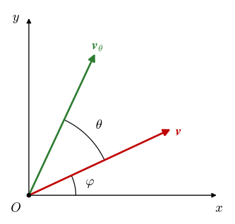
The angle \(\varphi\) disappears into the components \(v_x = |\bm v|\cos\varphi\) and \(v_y = |\bm v|\sin\varphi\), so one matrix turns every vector of the plane, \(\bm v_\theta = \bm R(\theta)\bm v\), and its columns are \(\bm R(\theta)\bm i\) and \(\bm R(\theta)\bm j\).
A turn by \(\theta\) followed by a turn by \(-\theta\) returns every vector to its place, which makes \(\bm R(-\theta)\) the inverse of \(\bm R(\theta)\). With \(\cos(-\theta) = \cos\theta\) and \(\sin(-\theta) = -\sin\theta\) the inverse is the transpose,
\[ \bm R(\theta)^{-1} = \bm R(-\theta) = \bm R(\theta)^\mathsf{T} \tag{3.13.2}\]
which makes \(\bm R(\theta)\) an orthogonal matrix in the sense of Chapter 3.11, with \(\det\bm R = \cos^2\theta + \sin^2\theta = 1\).
In SymPy we write the matrix once as a function of the angle and give the angle in radians, sp.rad(30) for \(30^\circ\).
def R(t):
# the columns are i and j turned by t
return sp.Matrix([[sp.cos(t), -sp.sin(t)],
[sp.sin(t), sp.cos(t)]])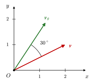
Turn \(\bm v = [2, 1]^\mathsf{T}\) in Figure 3.13.2 by \(30^\circ\) counterclockwise and check that the length and the angle come out right.
With \(\cos 30^\circ = \sqrt 3/2\) and \(\sin 30^\circ = 1/2\), 3.13.1 gives
\[ \bm v_\theta = \begin{bmatrix}\sqrt3/2 & -1/2\\ 1/2 & \sqrt3/2\end{bmatrix}\begin{bmatrix}2\\ 1\end{bmatrix} = \begin{bmatrix}\sqrt3 - 1/2\\ 1 + \sqrt3/2\end{bmatrix} \]
The length must stay \(|\bm v| = \sqrt 5\), and the angle between \(\bm v\) and \(\bm v_\theta\) follows from their dot product as in Chapter 3.6, \(\cos\alpha = \bm v\cdot\bm v_\theta/|\bm v|^2\).
vv = sp.Matrix([2, 1])
vv_th = R(sp.rad(30))*vv
length = sp.simplify(vv_th.norm())
cos_alpha = sp.simplify(vv.dot(vv_th)/vv.norm()**2)
The image, its length and the cosine of the angle turned are
\[ \begin{aligned}\bm v_\theta &= \left[\begin{matrix}- \dfrac{1}{2} + \sqrt{3}\\\dfrac{\sqrt{3}}{2} + 1\end{matrix}\right]\approx \left[\begin{matrix}1.232\\1.866\end{matrix}\right]\\ |\bm v_\theta| &= \sqrt{5}, \qquad \cos\alpha = \dfrac{\sqrt{3}}{2}\end{aligned} \]
The length is \(\sqrt 5\) and \(\cos\alpha = \sqrt3/2\) gives \(\alpha = 30^\circ\). The matrix turned the vector and changed nothing else.
Practise the plane rotation below. The fields accept expressions such as sqrt(3) - 1/2.
In space we turn about an axis. A turn about the \(z\) axis moves the \(x\) and \(y\) components exactly as in the plane and leaves \(v_z\) alone. Its matrix is 3.13.1 with a third row and column holding a 1 on the diagonal. The positive sense follows the right-hand rule of Chapter 3.7: with the thumb along the axis, the fingers curl the way a positive turn goes, which is counterclockwise when we look at the plane from the tip of the axis toward the origin.
The turns about \(x\) and \(y\) follow from the turn about \(z\) by renaming the axes in the cyclic order \(x\to y\to z\to x\). Seen from the tip of each axis, Figure 3.13.3, the turn about \(z\) carries \(x\) toward \(y\), the turn about \(x\) carries \(y\) toward \(z\), and the turn about \(y\) carries \(z\) toward \(x\). Each acts on its pair of axes with the pattern of 3.13.1, the \(-\sin\theta\) in the row of the first axis of the pair and the column of the second,
\[ \bm R_x(\theta) = \begin{bmatrix}1 & 0 & 0\\ 0 & \cos\theta & -\sin\theta\\ 0 & \sin\theta & \cos\theta\end{bmatrix},\quad \bm R_y(\theta) = \begin{bmatrix}\cos\theta & 0 & \sin\theta\\ 0 & 1 & 0\\ -\sin\theta & 0 & \cos\theta\end{bmatrix},\quad \bm R_z(\theta) = \begin{bmatrix}\cos\theta & -\sin\theta & 0\\ \sin\theta & \cos\theta & 0\\ 0 & 0 & 1\end{bmatrix} \tag{3.13.3}\]
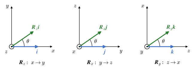
The minus sign of \(\bm R_y\) sits below the diagonal, which looks like a misprint and is not one. The pair of \(\bm R_y\) is \((z, x)\) in the cyclic order, and the \(-\sin\theta\) therefore belongs in row \(z\) and column \(x\); written with the rows in the order \(x\), \(y\), \(z\), that entry lands in the bottom left corner. The column check confirms it: \(\bm R_y(\theta)\bm k = [\sin\theta, 0, \cos\theta]^\mathsf{T}\), so a small positive turn about \(y\) tips \(\bm k\) toward \(+x\), as Figure 3.13.3 says.
The video turns a vector and the basis by \(90^\circ\) about \(x\), then \(y\), then \(z\), each time counterclockwise seen from the tip of the axis, and back.
In SymPy we write the three matrices of 3.13.3 as functions of the angle. SymPy’s own sp.rot_ccw_axis1(t), sp.rot_ccw_axis2(t) and sp.rot_ccw_axis3(t) return the same matrices.
def R_x(t):
    return sp.Matrix([[1, 0, 0],
                      [0, sp.cos(t), -sp.sin(t)],
                      [0, sp.sin(t),  sp.cos(t)]])

def R_y(t):
    # the pair is (z, x): z turns toward x, so -sin sits in row z, column x
    return sp.Matrix([[ sp.cos(t), 0, sp.sin(t)],
                      [0, 1, 0],
                      [-sp.sin(t), 0, sp.cos(t)]])

def R_z(t):
    return sp.Matrix([[sp.cos(t), -sp.sin(t), 0],
                      [sp.sin(t),  sp.cos(t), 0],
                      [0, 0, 1]])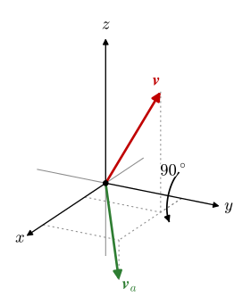
Turn \(\bm v = [1, 2, 3]^\mathsf{T}\) in Figure 3.13.4 by \(90^\circ\) about the \(y\) axis.
With \(\cos 90^\circ = 0\) and \(\sin 90^\circ = 1\), 3.13.3 gives
\[ \bm v_a = \bm R_y(90^\circ)\,\bm v = \begin{bmatrix}0 & 0 & 1\\ 0 & 1 & 0\\ -1 & 0 & 0\end{bmatrix}\begin{bmatrix}1\\ 2\\ 3\end{bmatrix} = \begin{bmatrix}3\\ 2\\ -1\end{bmatrix} \]
vv = sp.Matrix([1, 2, 3])
vv_a = R_y(sp.rad(90))*vv
SymPy agrees,
\[ \bm v_a = \bm R_y(90^\circ)\,\bm v = \left[\begin{matrix}3\\2\\-1\end{matrix}\right] \]
The \(y\) component stays 2. The \(z\) component 3 has moved to \(+x\) and the \(x\) component 1 to \(-z\), as a quarter turn that carries \(z\) toward \(x\) must do.
Practise the turns about the coordinate axes below.
Two rotations in a row are one map, the product of their matrices, Chapter 3.10. When the vector is first turned by \(\bm R_1\) and then by \(\bm R_2\), the second matrix acts on the result of the first, \(\bm R_2(\bm R_1\bm v) = (\bm R_2\bm R_1)\bm v\), so the matrix of the first turn stands next to the vector and each later turn is written to its left. The matrix product does not commute, and neither do rotations in space.
The product of two rotations is again a rotation. It keeps lengths, since each factor does, and it is orthogonal with determinant one,
\[ (\bm R_2\bm R_1)^\mathsf{T}(\bm R_2\bm R_1) = \bm R_1^\mathsf{T}\bm R_2^\mathsf{T}\bm R_2\bm R_1 = \bm R_1^\mathsf{T}\bm R_1 = \bm I, \qquad \det(\bm R_2\bm R_1) = \det\bm R_2\det\bm R_1 = 1 \]
with the transpose of a product from Chapter 3.10 and the determinant of a product from Chapter 3.11. The same check in SymPy, for \(\bm R_y\) with a symbolic angle,
th = sp.symbols('theta', real=True)
RR = R_y(th)
check_orth = sp.simplify(RR.T*RR)
check_det = sp.simplify(RR.det())
gives
\[ \bm R_y^\mathsf{T}\bm R_y = \left[\begin{matrix}1 & 0 & 0\\0 & 1 & 0\\0 & 0 & 1\end{matrix}\right], \qquad \det\bm R_y = 1 \]
An orthogonal matrix with determinant \(-1\) also keeps lengths, but it mirrors space, and a right-handed basis comes out left-handed. Determinant one is what separates a rotation from a reflection.
Here every turn is about a fixed axis of the coordinate system. A robot arm turns each joint about an axis that the earlier joints have carried along, and Chapter 6.2 shows that such a turn multiplies from the right.
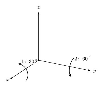
Find the matrix of the map that first turns by \(30^\circ\) about the \(x\) axis and then by \(60^\circ\) about the \(y\) axis, Figure 3.13.5. Compare it with the two turns in the reverse order.
The first turn stands next to the vector, so
\[ \bm v_a = \bm R_y(60^\circ)\,\bm R_x(30^\circ)\,\bm v, \qquad \bm v_b = \bm R_x(30^\circ)\,\bm R_y(60^\circ)\,\bm v \]
RR_a = R_y(sp.rad(60))*R_x(sp.rad(30))     # x first, then y
RR_b = R_x(sp.rad(30))*R_y(sp.rad(60))     # y first, then x
The two products are
\[ \begin{aligned}\bm R_y(60^\circ)\,\bm R_x(30^\circ) &= \left[\begin{matrix}\dfrac{1}{2} & \dfrac{\sqrt{3}}{4} & \dfrac{3}{4}\\0 & \dfrac{\sqrt{3}}{2} & - \dfrac{1}{2}\\- \dfrac{\sqrt{3}}{2} & \dfrac{1}{4} & \dfrac{\sqrt{3}}{4}\end{matrix}\right]\\ \bm R_x(30^\circ)\,\bm R_y(60^\circ) &= \left[\begin{matrix}\dfrac{1}{2} & 0 & \dfrac{\sqrt{3}}{2}\\\dfrac{\sqrt{3}}{4} & \dfrac{\sqrt{3}}{2} & - \dfrac{1}{4}\\- \dfrac{3}{4} & \dfrac{1}{2} & \dfrac{\sqrt{3}}{4}\end{matrix}\right]\end{aligned} \]
The two maps agree only on the diagonal. Both are rotations, each with \(\bm R^\mathsf{T}\bm R = \bm I\) and \(\det\bm R = 1\), but they leave a body in different places, as the video shows.
Practise two quarter turns in a row below. The answer sheet also gives the result in the reverse order.
A vector does not depend on the axes we measure it with, but its components do. Let \(\bm i\), \(\bm j\), \(\bm k\) and \(\bm i'\), \(\bm j'\), \(\bm k'\) be two bases in space, Figure 3.13.6 for the plane. The same vector \(\bm v\) is written in both,
\[ \bm v = v_x\bm i + v_y\bm j + v_z\bm k = v_{x'}\bm i' + v_{y'}\bm j' + v_{z'}\bm k' \]
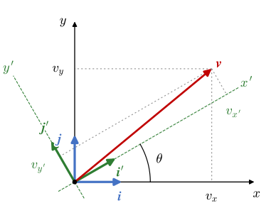
To relate the two sets of components we need the new basis vectors in the old components,
\[ \bm i' = t_{11}\bm i + t_{21}\bm j + t_{31}\bm k, \qquad \bm j' = t_{12}\bm i + t_{22}\bm j + t_{32}\bm k, \qquad \bm k' = t_{13}\bm i + t_{23}\bm j + t_{33}\bm k \]
Inserting these on the right and collecting the terms in \(\bm i\), \(\bm j\) and \(\bm k\) gives three equations, one per old component,
\[ \begin{aligned} v_x &= t_{11}v_{x'} + t_{12}v_{y'} + t_{13}v_{z'} \\ v_y &= t_{21}v_{x'} + t_{22}v_{y'} + t_{23}v_{z'} \\ v_z &= t_{31}v_{x'} + t_{32}v_{y'} + t_{33}v_{z'} \end{aligned} \]
or on matrix form \(\bm v = \bm T\bm v'\), where \(\bm v\) and \(\bm v'\) now stand for the columns of old and new components. The matrix \(\bm T = [\bm i'\ \bm j'\ \bm k']\) is the transformation matrix, and its columns are the new basis vectors written in the old basis. This is the column picture of Chapter 3.10: the old components are the combination of the new basis vectors weighted by the new components.
When both bases are orthonormal, the columns of \(\bm T\) are orthonormal and \(\bm T\) is orthogonal, \(\bm T^\mathsf{T}\bm T = \bm I\). Its inverse is its transpose, and the way back costs nothing,
\[ \bm v = \bm T\bm v' \quad\Longleftrightarrow\quad \bm v' = \bm T^\mathsf{T}\bm v, \qquad \bm T = [\bm i'\ \bm j'\ \bm k'] \tag{3.13.4}\]
Row by row, \(\bm T^\mathsf{T}\bm v\) holds the dot products of \(\bm v\) with the new basis vectors, \(v_{x'} = \bm i'\cdot\bm v\) and so on. Each new component is the cheap projection of \(\bm v\) on a unit vector from Chapter 3.6, and the rows of \(\bm T^\mathsf{T}\) are the unit vectors to project on.
When the new basis is the old one turned by \(\theta\) in the plane, its columns are those of 3.13.1, \(\bm T = \bm R(\theta)\), and by 3.13.2
\[ \bm v' = \bm R(\theta)^\mathsf{T}\bm v = \bm R(-\theta)\,\bm v \]
Turning the axes by \(\theta\) gives the same numbers as turning the vector by \(-\theta\) in fixed axes. In the video the axes turn on the left while the vector stays, and on the right the vector turns the other way in the fixed axes; the two readouts agree at every instant.
Grant Sanderson shows in the video below how a vector is translated between two bases that are neither orthogonal nor normalised, where \(\bm T^{-1}\) takes the place of \(\bm T^\mathsf{T}\). Its second half moves a whole map into the other basis, the subject of our last section.
sp.rot_axis1(t), sp.rot_axis2(t) and sp.rot_axis3(t) return the transposes \(\bm R_x(t)^\mathsf{T}\), \(\bm R_y(t)^\mathsf{T}\) and \(\bm R_z(t)^\mathsf{T}\) of 3.13.3. They give the components of a fixed vector in axes turned by \(t\), by 3.13.4. To turn the vector itself we use sp.rot_ccw_axis1(t) to sp.rot_ccw_axis3(t), or the functions written above. Other libraries make their own choice, and one column of a library’s matrix compared with Figure 3.13.3 tells which.
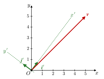
The new basis in Figure 3.13.7 is \(\bm i' = [3, 4]^\mathsf{T}/5\) and \(\bm j' = [-4, 3]^\mathsf{T}/5\). Find the components of \(\bm v = [5, 5]^\mathsf{T}\) in it.
Both basis vectors have length one and \(\bm i'\cdot\bm j' = 0\), so the basis is orthonormal and 3.13.4 applies with
\[ \bm T = [\bm i'\ \bm j'] = \frac15\begin{bmatrix}3 & -4\\ 4 & 3\end{bmatrix}, \qquad \bm v' = \bm T^\mathsf{T}\bm v = \frac15\begin{bmatrix}3 & 4\\ -4 & 3\end{bmatrix}\begin{bmatrix}5\\ 5\end{bmatrix} = \begin{bmatrix}7\\ -1\end{bmatrix} \]
and the check \(\bm T\bm v' = \bm v\) takes us back.
TT = sp.Matrix([[3, -4],
                [4,  3]])/5          # columns i' and j'
vv = sp.Matrix([5, 5])
vv_p = TT.T*vv
back = TT*vv_p
The new components and the way back are
\[ \bm v' = \bm T^\mathsf{T}\bm v = \left[\begin{matrix}7\\-1\end{matrix}\right], \qquad \bm T\bm v' = \left[\begin{matrix}5\\5\end{matrix}\right] \]
In the new basis \(\bm v = 7\bm i' - \bm j'\): seven units along \(x'\) and one unit back along \(y'\), as Figure 3.13.7 shows with \(\bm v\) below the \(x'\) axis. The length is the same in both bases, \(\sqrt{49 + 1} = \sqrt{25 + 25}\).
Practise components in a turned basis below. The new basis vectors are drawn in green, and the projections of \(\bm v\) on them appear once the answer is right.
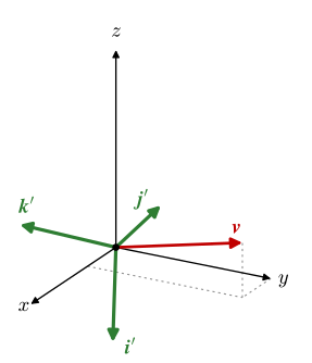
The basis in Figure 3.13.8 has
\[ \bm i' = \frac13\begin{bmatrix}2\\ 1\\ -2\end{bmatrix}, \qquad \bm j' = \frac13\begin{bmatrix}1\\ 2\\ 2\end{bmatrix}, \qquad \bm k' = \frac13\begin{bmatrix}2\\ -2\\ 1\end{bmatrix} \]
Check that it is orthonormal and right-handed, and find the components of \(\bm v = [1, 3, 1]^\mathsf{T}\) in it.
The three vectors are the columns of \(\bm T\). The basis is orthonormal when \(\bm T^\mathsf{T}\bm T = \bm I\), and right-handed when \(\det\bm T = 1\), the triple product of Chapter 3.7. The components are \(\bm v' = \bm T^\mathsf{T}\bm v\).
TT = sp.Matrix.hstack(sp.Matrix([2, 1, -2]),
                      sp.Matrix([1, 2, 2]),
                      sp.Matrix([2, -2, 1]))/3
vv = sp.Matrix([1, 3, 1])
vv_p = TT.T*vv
The two checks and the components are
\[ \begin{aligned}\bm T^\mathsf{T}\bm T &= \left[\begin{matrix}1 & 0 & 0\\0 & 1 & 0\\0 & 0 & 1\end{matrix}\right], \qquad \det\bm T = 1\\ \bm v' &= \bm T^\mathsf{T}\bm v = \left[\begin{matrix}1\\3\\-1\end{matrix}\right]\end{aligned} \]
The basis is orthonormal and right-handed, so \(\bm T\) is a rotation, and \(\bm v = \bm i' + 3\bm j' - \bm k'\). The middle component is the largest because \(\bm v\) lies closest to \(\bm j'\) in Figure 3.13.8.
The coordinates of a point are the components of its position vector, and that vector depends on the origin. Let the system \(O'x'y'z'\) have its origin at the point with the old coordinates \(\bm x_{O'}\) and the orthonormal basis \(\bm T = [\bm i'\ \bm j'\ \bm k']\). A point \(P\) has the coordinates \(\bm x\) in the old system and \(\bm x'\) in the new one. The vector from \(O\) to \(P\) is the vector from \(O\) to \(O'\) plus the vector from \(O'\) to \(P\). The first has the old components \(\bm x_{O'}\), the second has the new components \(\bm x'\) and by 3.13.4 the old components \(\bm T\bm x'\). Their sum gives
\[ \bm x = \bm x_{O'} + \bm T\bm x' \quad\Longleftrightarrow\quad \bm x' = \bm T^\mathsf{T}(\bm x - \bm x_{O'}) \tag{3.13.5}\]
The shift applies to points only. A vector between two points, such as \(\bm x_Q - \bm x_P\), loses \(\bm x_{O'}\) in the difference and changes by 3.13.4 alone.
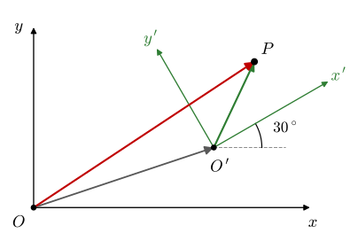
The point \(P\) in Figure 3.13.9 has the coordinates \((1.3, 0.9)\) in the system \(O'x'y'\), whose origin lies at \((3, 1)\) and whose axes are turned \(30^\circ\) counterclockwise from \(x\) and \(y\). Find the coordinates of \(P\) in the system \(Oxy\), and check the way back.
The turned basis has \(\bm T = \bm R(30^\circ)\), and 3.13.5 gives
\[ \bm x = \begin{bmatrix}3\\ 1\end{bmatrix} + \begin{bmatrix}\cos 30^\circ & -\sin 30^\circ\\ \sin 30^\circ & \cos 30^\circ\end{bmatrix}\begin{bmatrix}1.3\\ 0.9\end{bmatrix} \]
With decimal data we compute in NumPy.
xx_O = np.array([3.0, 1.0])            # O' in the old system
th = np.radians(30)
TT = np.array([[np.cos(th), -np.sin(th)],
               [np.sin(th),  np.cos(th)]])
xx_p = np.array([1.3, 0.9])            # P in the new system
xx = xx_O + TT @ xx_p
xx_back = TT.T @ (xx - xx_O)
The point and the way back are
\[ \begin{aligned}\bm x &= \begin{bmatrix}3.67583 \\ 2.42942\end{bmatrix}\\ \bm T^\mathsf{T}(\bm x - \bm x_{O'}) &= \begin{bmatrix}1.3 \\ 0.9\end{bmatrix}\end{aligned} \]
\(P\) lies at \((3.676, 2.429)\), up and to the right of \(O'\) as in Figure 3.13.9, and the transpose returns the coordinates we started from.
Practise the coordinates of a point in a moved and turned system below.
A matrix \(\bm A\) maps the components of \(\bm x\) to those of \(\bm y = \bm A\bm x\), both in the old basis. In the new basis the same map has another matrix \(\bm A'\), with \(\bm y' = \bm A'\bm x'\). Both vectors change basis by 3.13.4, \(\bm x = \bm T\bm x'\) and \(\bm y = \bm T\bm y'\), so
\[ \bm T\bm y' = \bm A\bm T\bm x' \quad\Rightarrow\quad \bm y' = \bm T^\mathsf{T}\bm A\bm T\,\bm x' \]
after a multiplication from the left by \(\bm T^\mathsf{T}\). The matrix of the map in the new basis is
\[ \bm A' = \bm T^\mathsf{T}\bm A\bm T \tag{3.13.6}\]
Read from the right, it takes new components to old ones with \(\bm T\), applies the map in the old basis with \(\bm A\), and returns to new components with \(\bm T^\mathsf{T}\). For a basis that is not orthonormal \(\bm T^{-1}\) replaces \(\bm T^\mathsf{T}\). The two matrices describe one map and share what belongs to it: \(\det\bm A' = \det\bm T^\mathsf{T}\det\bm A\det\bm T = \det\bm A\), the area or volume factor of Chapter 3.11. The stress and strain matrices of Chapter 8.7 change with the frame by 3.13.6, and Chapter 8.8 draws that change in the plane.
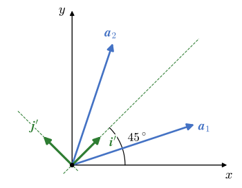
Find the matrix of \(\bm A = \begin{bmatrix}3 & 1\\ 1 & 3\end{bmatrix}\) in the basis turned \(45^\circ\), Figure 3.13.10.
The new basis is \(\bm T = \bm R(45^\circ) = \frac{1}{\sqrt2}\begin{bmatrix}1 & -1\\ 1 & 1\end{bmatrix}\), and 3.13.6 gives
\[ \bm A' = \frac12\begin{bmatrix}1 & 1\\ -1 & 1\end{bmatrix}\begin{bmatrix}3 & 1\\ 1 & 3\end{bmatrix}\begin{bmatrix}1 & -1\\ 1 & 1\end{bmatrix} = \frac12\begin{bmatrix}1 & 1\\ -1 & 1\end{bmatrix}\begin{bmatrix}4 & -2\\ 4 & 2\end{bmatrix} \]
AA = sp.Matrix([[3, 1],
                [1, 3]])
TT = R(sp.pi/4)
AA_p = sp.simplify(TT.T*AA*TT)
The matrix in the turned basis is
\[ \bm A' = \bm T^\mathsf{T}\bm A\bm T = \left[\begin{matrix}4 & 0\\0 & 2\end{matrix}\right], \qquad \det\bm A' = \det\bm A = 8 \]
In the turned basis the matrix is diagonal. The map stretches \(\bm i'\) by 4 and \(\bm j'\) by 2 and turns neither, which the matrix \(\bm A\) in the old basis hides. The determinant 8 and the trace 6 are the same in both bases. Chapter 3.14 finds such a basis for any symmetric matrix.
Practise a matrix in a turned basis below. Once the answer is right, the images \(\bm A\bm i'\) and \(\bm A\bm j'\) are drawn; their components along \(\bm i'\) and \(\bm j'\) are the columns of \(\bm A'\).