- 1
- A list of rows, each row a list of entries. Writing the rows on separate lines makes the code look like the matrix.
- 2
-
shapeis (rows, columns). Row index 1 and column index 2 are the second row and the third column.
((2, 3), 2)“It will be seen that matrices (attending only to those of the same order) comport themselves as single quantities; they may be added, multiplied or compounded together, &c.”
— Arthur Cayley, A memoir on the theory of matrices, 1858
A matrix is a rectangular table of numbers, its entries, arranged in rows and columns. A matrix with \(m\) rows and \(n\) columns is an \(m\times n\) matrix, and the entry in row \(i\) and column \(j\) is written \(a_{ij}\),
\[ \boxed{\bm A = \begin{bmatrix} a_{11} & a_{12} & \cdots & a_{1n} \\ a_{21} & a_{22} & \cdots & a_{2n} \\ \vdots & \vdots & \ddots & \vdots \\ a_{m1} & a_{m2} & \cdots & a_{mn} \end{bmatrix} = [a_{ij}]} \tag{3.10.1}\]
The first index counts the rows from the top and the second the columns from the left. A matrix with one column is a column vector, the form in which we have written every vector since Chapter 3.5, and a matrix with one row is a row vector. A \(1\times 1\) matrix is the number it holds.
A matrix also acts. Multiplied with a vector it returns a new vector, so it maps every point of the plane, or of space, to a new point. That reading decides how matrices are multiplied, and it is the one we keep in mind throughout.
Two matrices are equal, \(\bm A = \bm B\), when they have the same size and equal entries in every place, \(a_{ij} = b_{ij}\) for all \(i\) and \(j\). A matrix whose entries are all zero is a zero matrix, written \(\bm 0\). There is one zero matrix of each size, and two zero matrices of different sizes are different matrices.
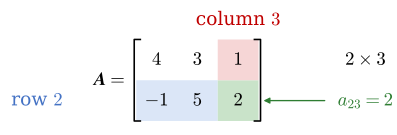
For the matrix \(\bm A\) in Figure 3.10.1, give the size, the entry \(a_{23}\), the second row and the third column, and set \(a_{13}\) to \(7\).
\(\bm A\) has two rows and three columns, so it is a \(2\times 3\) matrix. Row 2 and column 3 cross in \(a_{23} = 2\), and
\[ \text{row 2} = \begin{bmatrix} -1 & 5 & 2 \end{bmatrix}, \qquad \text{column 3} = \begin{bmatrix} 1 \\ 2 \end{bmatrix} \]
In Python the indices start at 0, so \(a_{23}\) is AA[1, 2]: one less than the mathematical index in both places. A colon in place of an index takes the whole row or column.
shape is (rows, columns). Row index 1 and column index 2 are the second row and the third column.
((2, 3), 2)1AA[1, :], AA[:, 2](Matrix([[-1, 5, 2]]),
Matrix([
[1],
[2]]))A list of indices picks several rows or columns in the order given, and an assignment changes the matrix in place:
1AA[[0, 1], [2, 0]]\(\displaystyle \left[\begin{matrix}1 & 4\\2 & -1\end{matrix}\right]\)
1AA[0, 2] = 7
AAAA.copy() would keep it.
\(\displaystyle \left[\begin{matrix}4 & 3 & 7\\-1 & 5 & 2\end{matrix}\right]\)
NumPy holds numbers in an array, built from the same list of rows, and indexes it the same way, with one difference: a single row or column comes back as a flat array of numbers, neither a row nor a column.
A = np.array([[4, 3, 1],
              [-1, 5, 2]])
1A.shape, A[1, 2], A[:, 2]array([1, 2]). A[:, 2:3] keeps it as a \(2\times 1\) array.
((2, 3), np.int64(2), array([1, 2]))We use SymPy matrices for exact work by hand and NumPy arrays once a problem is numerical, as in Basics of Python.
Two matrices of the same size are added entry by entry, and a number \(s\) multiplies every entry,
\[ \bm A + \bm B = [a_{ij} + b_{ij}], \qquad s\bm A = [s\,a_{ij}] \tag{3.10.2}\]
The difference is \(\bm A - \bm B = \bm A + (-1)\bm B\). Matrices of different sizes cannot be added. Because each entry follows the arithmetic of numbers, the sum and the scalar multiple obey the rules
\[ \begin{aligned} \bm A + \bm B &= \bm B + \bm A && \text{commutative law} \\ (\bm A + \bm B) + \bm C &= \bm A + (\bm B + \bm C) && \text{associative law} \\ \bm A + \bm 0 &= \bm A && \text{zero matrix} \\ s(\bm A + \bm B) &= s\bm A + s\bm B, \quad (s + t)\bm A = s\bm A + t\bm A && \text{distributive laws} \\ s(t\bm A) &= (st)\bm A && \text{associative law for scalars} \end{aligned} \]
for matrices \(\bm A\), \(\bm B\), \(\bm C\) of one size and numbers \(s\) and \(t\). These are the rules of vectors from Chapter 3.5, now for tables of any shape.

Compute \(\bm A + \bm B\), \(\bm A - \bm B\) and \(3\bm A\) for the two \(2\times 3\) matrices of Figure 3.10.2,
\[ \bm A = \begin{bmatrix} 2 & 5 & 4 \\ -1 & 3 & 0 \end{bmatrix}, \qquad \bm B = \begin{bmatrix} 1 & 2 & -2 \\ 11 & 8 & 7 \end{bmatrix} \]
Place by place,
\[ \begin{aligned} \bm A + \bm B &= \begin{bmatrix} 2 + 1 & 5 + 2 & 4 - 2 \\ -1 + 11 & 3 + 8 & 0 + 7 \end{bmatrix}, \\ \bm A - \bm B &= \begin{bmatrix} 2 - 1 & 5 - 2 & 4 + 2 \\ -1 - 11 & 3 - 8 & 0 - 7 \end{bmatrix}, \\ 3\bm A &= \begin{bmatrix} 3\cdot 2 & 3\cdot 5 & 3\cdot 4 \\ 3\cdot(-1) & 3\cdot 3 & 3\cdot 0 \end{bmatrix} \end{aligned} \]
AA = sp.Matrix([[2, 5, 4], [-1, 3, 0]])
BB = sp.Matrix([[1, 2, -2], [11, 8, 7]])
SymPy gives
\[ \bm A + \bm B = \left[\begin{matrix}3 & 7 & 2\\10 & 11 & 7\end{matrix}\right],\quad \bm A - \bm B = \left[\begin{matrix}1 & 3 & 6\\-12 & -5 & -7\end{matrix}\right],\quad 3\bm A = \left[\begin{matrix}6 & 15 & 12\\-3 & 9 & 0\end{matrix}\right] \]
Each result keeps the size \(2\times 3\) of its terms.
Every vector of the plane is a combination of the basis vectors, \(\bm x = x_1\bm i + x_2\bm j\). Consider a map \(T\) that sends each vector \(\bm x\) to a new vector \(T(\bm x)\) and that is linear: it keeps straight lines straight, keeps evenly spaced points on a line evenly spaced, and leaves the origin where it is. For vectors these requirements read
\[ T(\bm u + \bm v) = T(\bm u) + T(\bm v), \qquad T(s\bm u) = s\,T(\bm u) \]
and applied to \(\bm x\) they give
\[ T(\bm x) = x_1\,T(\bm i) + x_2\,T(\bm j) \]
A linear map is known as soon as we know where it sends \(\bm i\) and \(\bm j\). We write the two images as the columns of a matrix, \(\bm a_1 = T(\bm i)\) and \(\bm a_2 = T(\bm j)\), so that \(\bm A = [\bm a_1\ \bm a_2]\), and define the product of the matrix and a vector as this combination of its columns,
\[ \boxed{\bm A\bm x = \begin{bmatrix} a_{11} & a_{12} \\ a_{21} & a_{22} \end{bmatrix}\begin{bmatrix} x_1 \\ x_2 \end{bmatrix} = x_1\begin{bmatrix} a_{11} \\ a_{21} \end{bmatrix} + x_2\begin{bmatrix} a_{12} \\ a_{22} \end{bmatrix} = x_1\bm a_1 + x_2\bm a_2} \tag{3.10.3}\]
With \(\bm x = \bm i = [1, 0]^\mathsf{T}\) the combination is \(\bm a_1\), and with \(\bm x = \bm j\) it is \(\bm a_2\):
The columns of \(\bm A\) are where \(\bm i\) and \(\bm j\) land, \(\bm A\bm i = \bm a_1\) and \(\bm A\bm j = \bm a_2\).
Adding the two columns of 3.10.3 row by row gives the same vector in a second form,
\[ \bm A\bm x = \begin{bmatrix} a_{11}x_1 + a_{12}x_2 \\ a_{21}x_1 + a_{22}x_2 \end{bmatrix} \tag{3.10.4}\]
where each component is the dot product of a row of \(\bm A\) with \(\bm x\) (Chapter 3.6). The column form says what the map does, and the row form is the quicker one by hand. Nothing in the argument depends on the plane. An \(m\times n\) matrix has \(n\) columns with \(m\) components each, so \(\bm A\bm x = x_1\bm a_1 + \dots + x_n\bm a_n\) is defined when \(\bm x\) has \(n\) components, and the result has \(m\).
The video plays six maps of the plane. The faint fixed grid marks where the plane was and the blue grid where it goes. The matrix in the corner is read off the arrows \(\bm i\) and \(\bm j\) as they move, its columns being their tips, and \(\bm u\) and \(\bm v\) are carried along as \(\bm A\bm u\) and \(\bm A\bm v\). At every moment the grid lines stay straight and evenly spaced. The green unit square turns orange when a map turns the plane over, which Chapter 3.11 measures with the determinant.
| Map | Matrix |
|---|---|
| scaling by \(s\) | \(\begin{bmatrix} s & 0 \\ 0 & s \end{bmatrix}\) |
| stretch by \(s_1\) along \(x\) and \(s_2\) along \(y\) | \(\begin{bmatrix} s_1 & 0 \\ 0 & s_2 \end{bmatrix}\) |
| shear along \(x\) | \(\begin{bmatrix} 1 & k \\ 0 & 1 \end{bmatrix}\) |
| rotation by \(90^\circ\) | \(\begin{bmatrix} 0 & -1 \\ 1 & 0 \end{bmatrix}\) |
| reflection in the \(x\) axis | \(\begin{bmatrix} 1 & 0 \\ 0 & -1 \end{bmatrix}\) |
| projection on the \(x\) axis | \(\begin{bmatrix} 1 & 0 \\ 0 & 0 \end{bmatrix}\) |
Each matrix in Table 3.10.1 is read off the picture. The shear keeps \(\bm i\) and pushes \(\bm j\) sideways to \([k, 1]^\mathsf{T}\), and the projection sends \(\bm j\) to the zero vector, so its second column is zero and the whole plane falls onto the \(x\) axis.
Grant Sanderson tells the same story with other maps of the plane and shows how to read any \(2\times 2\) matrix as one.
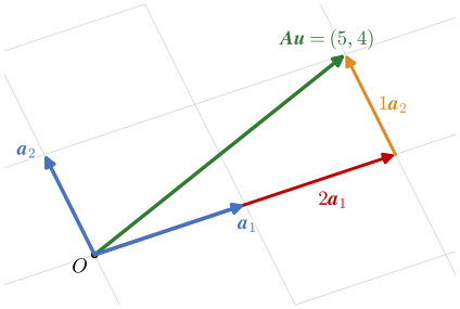
Find \(\bm A\bm u\) for
\[ \bm A = \begin{bmatrix} 3 & -1 \\ 1 & 2 \end{bmatrix}, \qquad \bm u = \begin{bmatrix} 2 \\ 1 \end{bmatrix} \]
as a combination of the columns of \(\bm A\) and by rows, Figure 3.10.3.
The columns are \(\bm a_1 = [3, 1]^\mathsf{T}\) and \(\bm a_2 = [-1, 2]^\mathsf{T}\), and 3.10.3 and 3.10.4 give
\[ \begin{aligned} \bm A\bm u &= 2\begin{bmatrix} 3 \\ 1 \end{bmatrix} + 1\begin{bmatrix} -1 \\ 2 \end{bmatrix} = \begin{bmatrix} 5 \\ 4 \end{bmatrix} \\ \bm A\bm u &= \begin{bmatrix} 3\cdot 2 + (-1)\cdot 1 \\ 1\cdot 2 + 2\cdot 1 \end{bmatrix} = \begin{bmatrix} 5 \\ 4 \end{bmatrix} \end{aligned} \]
In SymPy * between two matrices is the matrix product; with NumPy arrays the product is written @.
AA = sp.Matrix([[3, -1], [1, 2]])
uu = sp.Matrix([2, 1])
Au = AA*uu
Au_columns = uu[0]*AA[:, 0] + uu[1]*AA[:, 1]     # x1 a1 + x2 a2, built by hand
Au_np = np.array([[3, -1], [1, 2]]) @ np.array([2, 1])
The product, the combination of the columns and the NumPy result agree:
\[ \bm A\bm u = \left[\begin{matrix}5\\4\end{matrix}\right],\quad 2\bm a_1 + 1\bm a_2 = \left[\begin{matrix}5\\4\end{matrix}\right],\quad \texttt{A @ u} = \left[\begin{matrix}5\\4\end{matrix}\right] \]
In the video \(\bm u\) is drawn tip to tail as \(2\bm i\) followed by \(1\bm j\). As \(\bm A\) acts, the first part is carried to \(2\bm a_1\) and the second to \(1\bm a_2\). The map keeps the path a path, so it ends at \(\bm A\bm u\).
Practise the product of a matrix and a vector below. The Python switch turns the exercise into code: the same problem is solved with SymPy and checked when we run it.
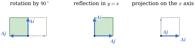
Find the matrices of the three maps in Figure 3.10.4: the rotation by \(90^\circ\) counterclockwise, the reflection in the line \(y = x\) and the projection on the \(x\) axis. Check each on \(\bm u = [3, 2]^\mathsf{T}\).
We read where \(\bm i\) and \(\bm j\) land and write the images as columns. The quarter turn sends \(\bm i\) to \(\bm j\) and \(\bm j\) to \(-\bm i\). The reflection in \(y = x\) swaps the two. The projection keeps \(\bm i\) and sends \(\bm j\) to \(\bm 0\). So
\[ \bm R = \begin{bmatrix} 0 & -1 \\ 1 & 0 \end{bmatrix}, \qquad \bm F = \begin{bmatrix} 0 & 1 \\ 1 & 0 \end{bmatrix}, \qquad \bm P = \begin{bmatrix} 1 & 0 \\ 0 & 0 \end{bmatrix} \]
and on \(\bm u\) the rotation should give \([-2, 3]^\mathsf{T}\), the reflection \([2, 3]^\mathsf{T}\) and the projection \([3, 0]^\mathsf{T}\).
ii, jj = sp.Matrix([1, 0]), sp.Matrix([0, 1])
# each matrix is built from the images of i and j, placed side by side as columns
RR = sp.Matrix.hstack(jj, -ii)
FF = sp.Matrix.hstack(jj, ii)
PP = sp.Matrix.hstack(ii, sp.zeros(2, 1))
uu = sp.Matrix([3, 2])
The three matrices and their action on \(\bm u\) are
\[ \begin{aligned}\bm R &= \left[\begin{matrix}0 & -1\\1 & 0\end{matrix}\right],\quad \bm F = \left[\begin{matrix}0 & 1\\1 & 0\end{matrix}\right],\quad \bm P = \left[\begin{matrix}1 & 0\\0 & 0\end{matrix}\right]\\ \bm R\bm u &= \left[\begin{matrix}-2\\3\end{matrix}\right],\quad \bm F\bm u = \left[\begin{matrix}2\\3\end{matrix}\right],\quad \bm P\bm u = \left[\begin{matrix}3\\0\end{matrix}\right]\end{aligned} \]
The rotation turns \(\bm u\) a quarter turn, the reflection swaps its components and the projection drops the \(y\) component, as the pictures promise.
Practise reading a matrix off its picture below.
A system of linear equations asks the opposite question: which \(\bm x\) does \(\bm A\) send to a given vector \(\bm b\)? Chapter 3.12 answers it.
Let \(\bm B\) act first and \(\bm A\) second. A vector \(\bm x\) goes to \(\bm B\bm x\) and then to \(\bm A(\bm B\bm x)\). Two linear maps in sequence form a linear map, and by 3.10.3 its matrix has as columns the images of the basis vectors. The first one is \(\bm A(\bm B\bm i) = \bm A\bm b_1\), where \(\bm b_1\) is the first column of \(\bm B\), and so on. We call that matrix the product \(\bm A\bm B\),
\[ \boxed{\bm A\bm B = \bm A\,[\bm b_1\ \bm b_2\ \cdots\ \bm b_n] = [\bm A\bm b_1\ \bm A\bm b_2\ \cdots\ \bm A\bm b_n]} \tag{3.10.5}\]
so that \((\bm A\bm B)\bm x = \bm A(\bm B\bm x)\) for every \(\bm x\). A product of maps is read from right to left: the factor next to \(\bm x\) acts first.
Entry \(c_{ij}\) of \(\bm C = \bm A\bm B\) sits in column \(j\), which is \(\bm A\bm b_j\), and by 3.10.4 its component \(i\) is the dot product of row \(i\) of \(\bm A\) with column \(j\) of \(\bm B\),
\[ c_{ij} = a_{i1}b_{1j} + a_{i2}b_{2j} + \dots + a_{ip}b_{pj} = \sum_{k=1}^{p} a_{ik}b_{kj} \tag{3.10.6}\]
the rule of row times column. A row of \(\bm A\) and a column of \(\bm B\) can only be paired when they have equally many entries, so \(\bm A\bm B\) is defined only when \(\bm A\) has as many columns as \(\bm B\) has rows. The result has the rows of \(\bm A\) and the columns of \(\bm B\):
\[ (m\times p)\,(p\times n) = m\times n \]
Grant Sanderson builds the product from two maps in sequence and computes it column by column.
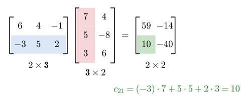
Compute \(\bm A\bm B\) and \(\bm B\bm A\) for
\[ \bm A = \begin{bmatrix} 6 & 4 & -1 \\ -3 & 5 & 2 \end{bmatrix}, \qquad \bm B = \begin{bmatrix} 7 & 4 \\ 5 & -8 \\ 3 & 6 \end{bmatrix} \]
By the size rule \((2\times 3)(3\times 2) = 2\times 2\) and \((3\times 2)(2\times 3) = 3\times 3\), so both products are defined, Figure 3.10.5. Row times column, 3.10.6, gives
\[ \begin{aligned} \bm A\bm B &= \begin{bmatrix} 6\cdot 7 + 4\cdot 5 + (-1)\cdot 3 & 6\cdot 4 + 4\cdot(-8) + (-1)\cdot 6 \\ (-3)\cdot 7 + 5\cdot 5 + 2\cdot 3 & (-3)\cdot 4 + 5\cdot(-8) + 2\cdot 6 \end{bmatrix} = \begin{bmatrix} 59 & -14 \\ 10 & -40 \end{bmatrix} \\ \bm B\bm A &= \begin{bmatrix} 7\cdot 6 + 4\cdot(-3) & 7\cdot 4 + 4\cdot 5 & 7\cdot(-1) + 4\cdot 2 \\ 5\cdot 6 + (-8)(-3) & 5\cdot 4 + (-8)\cdot 5 & 5\cdot(-1) + (-8)\cdot 2 \\ 3\cdot 6 + 6\cdot(-3) & 3\cdot 4 + 6\cdot 5 & 3\cdot(-1) + 6\cdot 2 \end{bmatrix} \end{aligned} \]
AA = sp.Matrix([[6, 4, -1], [-3, 5, 2]])
BB = sp.Matrix([[7, 4], [5, -8], [3, 6]])
AB = AA*BB
BA = BB*AA
SymPy completes both products:
\[ \bm A\bm B = \left[\begin{matrix}59 & -14\\10 & -40\end{matrix}\right],\qquad \bm B\bm A = \left[\begin{matrix}30 & 48 & 1\\54 & -20 & -21\\0 & 42 & 9\end{matrix}\right] \]
Both products exist, and they are not even of the same size: \(\bm A\bm B \neq \bm B\bm A\).
NumPy writes the matrix product with the operator @. The star * also works on two arrays, but it multiplies entry by entry:
A = np.array([[6, 4, -1], [-3, 5, 2]])
B = np.array([[7, 4], [5, -8], [3, 6]])
1A @ Barray([[ 59, -14],
[ 10, -40]])1A * A* returns a \(2\times 3\) result.
array([[36, 16,  1],
[ 9, 25, 4]])@ and * with NumPy arrays
For NumPy arrays A @ B is the matrix product and A * B the entry-by-entry product. With two square arrays of one size both return a matrix of that size, and no error tells us which one we computed. With SymPy matrices * is the matrix product, and @ gives the same. We write @ with every NumPy array and read every * between two arrays as a possible error.
Practise row times column below. Clicking into an entry field lights the row and the column that make it.
For matrices whose sizes allow the products and for a number \(s\),
\[ \begin{aligned} (\bm A\bm B)\bm C &= \bm A(\bm B\bm C) && \text{associative law} \\ \bm A(\bm B + \bm C) &= \bm A\bm B + \bm A\bm C && \text{distributive law from the left} \\ (\bm A + \bm B)\bm C &= \bm A\bm C + \bm B\bm C && \text{distributive law from the right} \\ s(\bm A\bm B) &= (s\bm A)\bm B = \bm A(s\bm B) && \text{scalar factor} \end{aligned} \tag{3.10.7}\]
The associative law needs no computation in the picture of maps: both sides apply \(\bm C\), then \(\bm B\), then \(\bm A\). So brackets in a product may be dropped, \(\bm A\bm B\bm C\), but the order of the factors may not be changed, since in general
\[ \bm A\bm B \neq \bm B\bm A \]
When the two products happen to be equal, \(\bm A\) and \(\bm B\) are said to commute. A second habit from numbers also fails: \(\bm A\bm B = \bm 0\) does not need a zero factor. Projecting on the \(x\) axis and then on the \(y\) axis sends every vector of the plane to \(\bm 0\), although neither projection is the zero matrix.
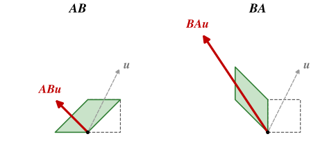
Let \(\bm A\) be the shear and \(\bm B\) the quarter turn,
\[ \bm A = \begin{bmatrix} 1 & 1 \\ 0 & 1 \end{bmatrix}, \qquad \bm B = \begin{bmatrix} 0 & -1 \\ 1 & 0 \end{bmatrix} \]
Find the matrices of the quarter turn followed by the shear and of the shear followed by the quarter turn, and the images of \(\bm u = [1, 2]^\mathsf{T}\), Figure 3.10.6.
The quarter turn first is \(\bm A\bm B\), the factor next to \(\bm u\) acting first. By 3.10.5 its columns are \(\bm A\) times the columns of \(\bm B\), and those of \(\bm B\bm A\) are \(\bm B\) times the columns of \(\bm A\),
\[ \begin{aligned} \bm A\bm B &= \left[\bm A\begin{bmatrix} 0 \\ 1 \end{bmatrix}\ \bm A\begin{bmatrix} -1 \\ 0 \end{bmatrix}\right] = \begin{bmatrix} 1 & -1 \\ 1 & 0 \end{bmatrix} \\ \bm B\bm A &= \left[\bm B\begin{bmatrix} 1 \\ 0 \end{bmatrix}\ \bm B\begin{bmatrix} 1 \\ 1 \end{bmatrix}\right] = \begin{bmatrix} 0 & -1 \\ 1 & 1 \end{bmatrix} \end{aligned} \]
AA = sp.Matrix([[1, 1], [0, 1]])
BB = sp.Matrix([[0, -1], [1, 0]])
uu = sp.Matrix([1, 2])
The two products and the two images of \(\bm u\) are
\[ \begin{aligned}\bm A\bm B &= \left[\begin{matrix}1 & -1\\1 & 0\end{matrix}\right],\quad \bm A\bm B\bm u = \left[\begin{matrix}-1\\1\end{matrix}\right]\\ \bm B\bm A &= \left[\begin{matrix}0 & -1\\1 & 1\end{matrix}\right],\quad \bm B\bm A\bm u = \left[\begin{matrix}-2\\3\end{matrix}\right]\end{aligned} \]
The same two maps in the other order send \(\bm u\) to a different point. The video plays both orders, and the dashed outline keeps the result of the first while the second is played.
The transpose \(\bm A^\mathsf{T}\) of an \(m\times n\) matrix \(\bm A\) is the \(n\times m\) matrix whose rows are the columns of \(\bm A\), entry by entry \((\bm A^\mathsf{T})_{ij} = a_{ji}\). For instance
\[ \begin{bmatrix} 2 & 5 & 4 \\ -1 & 3 & 0 \end{bmatrix}^\mathsf{T} = \begin{bmatrix} 2 & -1 \\ 5 & 3 \\ 4 & 0 \end{bmatrix} \]
The transpose obeys
\[ \begin{aligned} (\bm A^\mathsf{T})^\mathsf{T} &= \bm A, \qquad (\bm A + \bm B)^\mathsf{T} = \bm A^\mathsf{T} + \bm B^\mathsf{T}, \qquad (s\bm A)^\mathsf{T} = s\bm A^\mathsf{T} \\ (\bm A\bm B)^\mathsf{T} &= \bm B^\mathsf{T}\bm A^\mathsf{T} \end{aligned} \tag{3.10.8}\]
and the last rule reverses the order. Entry \(ij\) of \((\bm A\bm B)^\mathsf{T}\) is entry \(ji\) of \(\bm A\bm B\), and by 3.10.6
\[ \big((\bm A\bm B)^\mathsf{T}\big)_{ij} = \sum_k a_{jk}b_{ki} = \sum_k (\bm B^\mathsf{T})_{ik}(\bm A^\mathsf{T})_{kj} = (\bm B^\mathsf{T}\bm A^\mathsf{T})_{ij} \]
The sizes demand the reversal as well: with \(\bm A\) of size \(m\times p\) and \(\bm B\) of size \(p\times n\), the product \(\bm B^\mathsf{T}\bm A^\mathsf{T}\) is \((n\times p)(p\times m)\), while \(\bm A^\mathsf{T}\bm B^\mathsf{T}\) is in general not defined.
A column vector is an \(n\times 1\) matrix, and its transpose is a row. The product of the row \(\bm a^\mathsf{T}\) and the column \(\bm b\) is a \(1\times 1\) matrix, row times column,
\[ \bm a^\mathsf{T}\bm b = \begin{bmatrix} a_1 & a_2 & a_3 \end{bmatrix}\begin{bmatrix} b_1 \\ b_2 \\ b_3 \end{bmatrix} = a_1b_1 + a_2b_2 + a_3b_3 = \bm a\cdot\bm b \tag{3.10.9}\]
the dot product of Chapter 3.6 written as a matrix product. In SymPy the transpose is .T. With the matrices of Example 5 and with \(\bm a = [2, 1, 3]^\mathsf{T}\) and \(\bm b = [1, -1, 2]^\mathsf{T}\) we check the product rule and 3.10.9:
AA = sp.Matrix([[6, 4, -1], [-3, 5, 2]])
BB = sp.Matrix([[7, 4], [5, -8], [3, 6]])
rule = (AA*BB).T - BB.T*AA.T          # the zero matrix if the rule holds

aa = sp.Matrix([2, 1, 3])
bb = sp.Matrix([1, -1, 2])
aTb = aa.T*bb                         # a 1x1 matrix
which gives
\[ (\bm A\bm B)^\mathsf{T} - \bm B^\mathsf{T}\bm A^\mathsf{T} = \left[\begin{matrix}0 & 0\\0 & 0\end{matrix}\right],\qquad \bm a^\mathsf{T}\bm b = \left[\begin{matrix}7\end{matrix}\right],\qquad \bm a\cdot\bm b = 7 \]
The product aa.T*bb is the \(1\times 1\) matrix \([7]\), and aTb[0] takes out the number.
An \(n\times n\) matrix is square. Its entries \(a_{11}, a_{22}, \dots, a_{nn}\) form the main diagonal. A square matrix with only zeros below the diagonal is upper triangular, one with only zeros above it lower triangular,
\[ \begin{bmatrix} 2 & 5 & 9 \\ 0 & 7 & 1 \\ 0 & 0 & 3 \end{bmatrix}, \qquad \begin{bmatrix} 7 & 0 & 0 & 0 \\ 1 & 5 & 0 & 0 \\ 8 & 9 & 4 & 0 \\ -1 & 3 & 5 & 3 \end{bmatrix} \]
A square matrix is symmetric when \(\bm A^\mathsf{T} = \bm A\), that is \(a_{ji} = a_{ij}\): the diagonal is a mirror for the entries. It is antisymmetric when \(\bm A^\mathsf{T} = -\bm A\). On the diagonal that reads \(a_{ii} = -a_{ii}\), so an antisymmetric matrix has zeros there. Every square matrix splits into a symmetric part and an antisymmetric part,
\[ \bm A = \underbrace{\tfrac12(\bm A + \bm A^\mathsf{T})}_{\bm S} + \underbrace{\tfrac12(\bm A - \bm A^\mathsf{T})}_{\bm K} \tag{3.10.10}\]
and the rules 3.10.8 confirm the two parts, \(\bm S^\mathsf{T} = \tfrac12(\bm A^\mathsf{T} + \bm A) = \bm S\) and \(\bm K^\mathsf{T} = \tfrac12(\bm A^\mathsf{T} - \bm A) = -\bm K\).
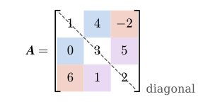
Split the matrix of Figure 3.10.7,
\[ \bm A = \begin{bmatrix} 1 & 4 & -2 \\ 0 & 3 & 5 \\ 6 & 1 & 2 \end{bmatrix} \]
into a symmetric and an antisymmetric part.
By 3.10.10 each entry of \(\bm S\) is the mean of a mirrored pair, \(s_{ij} = \tfrac12(a_{ij} + a_{ji})\), and each entry of \(\bm K\) half their difference, \(k_{ij} = \tfrac12(a_{ij} - a_{ji})\). The pair \(a_{12} = 4\), \(a_{21} = 0\) gives \(s_{12} = 2\) and \(k_{12} = 2\), and in the same way
\[ \bm S = \begin{bmatrix} 1 & 2 & 2 \\ 2 & 3 & 3 \\ 2 & 3 & 2 \end{bmatrix}, \qquad \bm K = \begin{bmatrix} 0 & 2 & -4 \\ -2 & 0 & 2 \\ 4 & -2 & 0 \end{bmatrix} \]
AA = sp.Matrix([[1, 4, -2], [0, 3, 5], [6, 1, 2]])
SS = (AA + AA.T)/2
KK = (AA - AA.T)/2
SymPy gives the two parts, and they add up to \(\bm A\):
\[ \bm S = \left[\begin{matrix}1 & 2 & 2\\2 & 3 & 3\\2 & 3 & 2\end{matrix}\right],\quad \bm K = \left[\begin{matrix}0 & 2 & -4\\-2 & 0 & 2\\4 & -2 & 0\end{matrix}\right],\quad \bm S + \bm K - \bm A = \left[\begin{matrix}0 & 0 & 0\\0 & 0 & 0\\0 & 0 & 0\end{matrix}\right] \]
\(\bm S\) keeps the diagonal of \(\bm A\) and \(\bm K\) has zeros there, as an antisymmetric matrix must.
Practise the split below.
One symmetric matrix appears so often that it deserves its own line. For any matrix \(\bm A\), square or not, the products \(\bm A^\mathsf{T}\bm A\) and \(\bm A\bm A^\mathsf{T}\) are square and symmetric, since by 3.10.8
\[ (\bm A^\mathsf{T}\bm A)^\mathsf{T} = \bm A^\mathsf{T}(\bm A^\mathsf{T})^\mathsf{T} = \bm A^\mathsf{T}\bm A \]
and likewise for \(\bm A\bm A^\mathsf{T}\). Entry \(ij\) of \(\bm A^\mathsf{T}\bm A\) is the dot product of columns \(i\) and \(j\) of \(\bm A\). The sum of the diagonal entries of a square matrix is its trace, \(\operatorname{tr}\bm A = a_{11} + a_{22} + \dots + a_{nn}\). For the \(2\times 3\) matrix of Example 2 the two products have different sizes:
AA = sp.Matrix([[2, 5, 4], [-1, 3, 0]])
AAT = AA*AA.T
ATA = AA.T*AA
Both are symmetric, and their traces are equal,
\[ \bm A\bm A^\mathsf{T} = \left[\begin{matrix}45 & 13\\13 & 10\end{matrix}\right],\quad \bm A^\mathsf{T}\bm A = \left[\begin{matrix}5 & 7 & 8\\7 & 34 & 20\\8 & 20 & 16\end{matrix}\right],\quad \operatorname{tr}\bm A\bm A^\mathsf{T} = 55,\quad \operatorname{tr}\bm A^\mathsf{T}\bm A = 55 \]
Each diagonal entry of \(\bm A^\mathsf{T}\bm A\) is a column dotted with itself, so both traces are the sum of the squares of all entries of \(\bm A\), here \(4 + 25 + 16 + 1 + 9 + 0 = 55\). The product \(\bm A^\mathsf{T}\bm A\) returns in Chapter 3.15.
A square matrix whose entries off the diagonal are all zero is a diagonal matrix, written \(\bm D = \operatorname{diag}(d_1, d_2, \dots, d_n)\). As a map it stretches each axis by its own factor, the stretch of Table 3.10.1. The diagonal matrix with ones on the diagonal is the identity matrix \(\bm I\). Its columns are the basis vectors themselves, so it leaves every vector where it is, and for every \(\bm A\) of a fitting size
\[ \bm A\bm I = \bm I\bm A = \bm A \]
\(\bm I\) plays the part of the number 1. There is one identity matrix of each size, and \(\bm I\bm A\) and \(\bm A\bm I\) use different ones when \(\bm A\) is not square.
A diagonal matrix multiplies in a simple pattern. By 3.10.6 the sum in \((\bm D\bm A)_{ij}\) keeps only the term \(k = i\), and the sum in \((\bm A\bm D)_{ij}\) only the term \(k = j\),
\[ (\bm D\bm A)_{ij} = d_i\,a_{ij}, \qquad (\bm A\bm D)_{ij} = a_{ij}\,d_j \tag{3.10.11}\]
From the left, \(\bm D\) multiplies row \(i\) of \(\bm A\) by \(d_i\). From the right, it multiplies column \(j\) by \(d_j\).
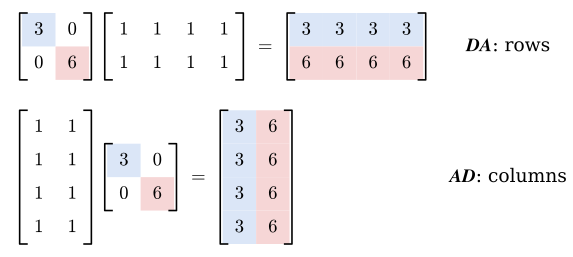
With \(\bm D = \operatorname{diag}(3, 6)\), compute \(\bm D\bm A\) for the \(2\times 4\) matrix \(\bm A\) of ones and \(\bm A\bm D\) for the \(4\times 2\) matrix of ones, Figure 3.10.8.
By 3.10.11 the first product has rows of 3 and of 6, and the second has columns of 3 and of 6.
DD = sp.diag(3, 6)
DA = DD*sp.ones(2, 4)
AD = sp.ones(4, 2)*DD
The two products are
\[ \bm D\bm A = \left[\begin{matrix}3 & 3 & 3 & 3\\6 & 6 & 6 & 6\end{matrix}\right],\qquad \bm A\bm D = \left[\begin{matrix}3 & 6\\3 & 6\\3 & 6\\3 & 6\end{matrix}\right] \]
The same diagonal matrix scales rows from one side and columns from the other.
Practise both sides below.
A square matrix can be multiplied by itself, and its powers are defined as for numbers,
\[ \bm A^0 = \bm I, \qquad \bm A^n = \bm A\,\bm A^{n-1}, \quad n = 1, 2, \dots \]
so that \(\bm A^2 = \bm A\bm A\) and \(\bm A^3 = \bm A\bm A\bm A\). As a map, \(\bm A^n\) applies \(\bm A\) \(n\) times. The laws \(\bm A^m\bm A^n = \bm A^{m + n}\) and \((\bm A^m)^n = \bm A^{mn}\) hold, since all the factors are the same matrix and the order cannot matter.
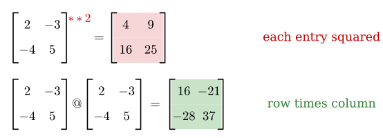
A**2 on a NumPy array squares each entry, A @ A multiplies row by column.
Compute \(\bm A^2\) and \(\bm A^{15}\) for
\[ \bm A = \begin{bmatrix} 2 & -3 \\ -4 & 5 \end{bmatrix} \]
By row times column,
\[ \bm A^2 = \begin{bmatrix} 2\cdot 2 + (-3)(-4) & 2\cdot(-3) + (-3)\cdot 5 \\ (-4)\cdot 2 + 5\cdot(-4) & (-4)(-3) + 5\cdot 5 \end{bmatrix} = \begin{bmatrix} 16 & -21 \\ -28 & 37 \end{bmatrix} \]
and \(\bm A^{15}\) is left to the computer. In SymPy AA**15 is the matrix power. On a NumPy array **, like *, acts entry by entry, Figure 3.10.9, and the matrix power is np.linalg.matrix_power.
AA = sp.Matrix([[2, -3], [-4, 5]])
A = np.array([[2, -3], [-4, 5]])
A2_np = np.linalg.matrix_power(A, 2)    # the matrix power, the same as A @ A
A2_entries = A**2                       # each entry squared: no power of the matrix
SymPy and matrix_power agree on \(\bm A^2\), while A**2 squares each entry:
\[ \bm A^2 = \left[\begin{matrix}16 & -21\\-28 & 37\end{matrix}\right],\quad \texttt{matrix\_power(A, 2)} = \left[\begin{matrix}16 & -21\\-28 & 37\end{matrix}\right],\quad \texttt{A**2} = \left[\begin{matrix}4 & 9\\16 & 25\end{matrix}\right] \]
The fifteenth power is
\[ \bm A^{15} = \left[\begin{matrix}2549464720604 & -3362053837617\\-4482738450156 & 5911518558221\end{matrix}\right] \]
The entries grow fast, because \(\bm A\) stretches some directions by a factor of about 7 and each power applies that stretch once more; Chapter 3.14 finds that direction and factor.
When the entries of a matrix are functions of a variable \(x\), the matrix is a function of \(x\) too, \(\bm A(x) = [a_{ij}(x)]\), as a vector function was a function of its parameter in Chapter 3.9. Its derivative and its integral are taken entry by entry,
\[ \frac{\mathrm d\bm A}{\mathrm dx} = \left[\frac{\mathrm da_{ij}}{\mathrm dx}\right], \qquad \int\bm A\,\mathrm dx = \left[\int a_{ij}\,\mathrm dx\right] \tag{3.10.12}\]
and the rules of the derivative carry over, with one care: in the product rule
\[ \frac{\mathrm d}{\mathrm dx}(\bm A\bm B) = \frac{\mathrm d\bm A}{\mathrm dx}\bm B + \bm A\frac{\mathrm d\bm B}{\mathrm dx} \]
each term keeps the factors in their order.
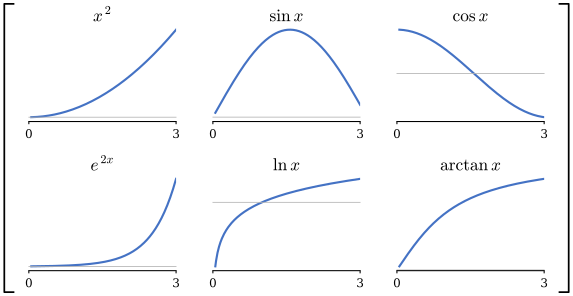
Differentiate and integrate the matrix of Figure 3.10.10,
\[ \bm A(x) = \begin{bmatrix} x^2 & \sin x & \cos x \\ e^{2x} & \ln x & \arctan x \end{bmatrix}, \qquad x > 0 \]
By 3.10.12 each entry is treated on its own, and SymPy’s diff and integrate act on each entry of a matrix.
x = sp.symbols('x', positive=True)     # positive, so that ln x is defined
AA = sp.Matrix([[x**2, sp.sin(x), sp.cos(x)],
                [sp.exp(2*x), sp.log(x), sp.atan(x)]])
dA = AA.diff(x)
intA = AA.integrate(x)
The derivative and an antiderivative are
\[ \begin{aligned}\frac{\mathrm d\bm A}{\mathrm dx} &= \left[\begin{matrix}2 x & \cos{\left(x \right)} & - \sin{\left(x \right)}\\2 e^{2 x} & \dfrac{1}{x} & \dfrac{1}{x^{2} + 1}\end{matrix}\right]\\ \int\bm A\,\mathrm dx &= \left[\begin{matrix}\dfrac{x^{3}}{3} & - \cos{\left(x \right)} & \sin{\left(x \right)}\\\dfrac{e^{2 x}}{2} & x \log{\left(x \right)} - x & x \operatorname{atan}{\left(x \right)} - \dfrac{\log{\left(x^{2} + 1 \right)}}{2}\end{matrix}\right]\end{aligned} \]
SymPy leaves out the constant of integration, one for each entry, as it does for a single function.
Everything above holds in space. A \(3\times 3\) matrix has three columns, the images of \(\bm i\), \(\bm j\) and \(\bm k\), and by 3.10.3 it sends \(\bm x = x_1\bm i + x_2\bm j + x_3\bm k\) to \(x_1\bm a_1 + x_2\bm a_2 + x_3\bm a_3\). In the video the unit cube is carried by
\[ \bm A = \begin{bmatrix} 1 & 1 & 0 \\ 0 & 2 & 0 \\ 1 & 0 & 1 \end{bmatrix} \]
Its edges stay straight and parallel, and its three edges from the origin end on the three columns of \(\bm A\); \(\bm k\) stays where it was, since the third column is \(\bm k\).
A matrix need not be square. A \(3\times 2\) matrix has two columns with three components each: it sends the two basis vectors of the plane to two vectors in space, and the whole plane to the plane through the origin that those two columns span. A \(2\times 3\) matrix goes the other way, from space to the plane. The simplest one drops the \(z\) component,
\[ \begin{bmatrix} 1 & 0 & 0 \\ 0 & 1 & 0 \end{bmatrix}\begin{bmatrix} x_1 \\ x_2 \\ x_3 \end{bmatrix} = \begin{bmatrix} x_1 \\ x_2 \end{bmatrix} \]
the view of space from above. The size rule \((m\times n)(n\times 1) = m\times 1\) states the same: the matrix takes vectors with as many components as it has columns and returns vectors with as many components as it has rows.