Code
x, y, z, t = sp.symbols('x y z t', real=True)
rr_P1 = sp.Matrix([2, 4, -1])
rr_P2 = sp.Matrix([5, 0, 7])

rr_0 = rr_P1
vv = rr_P2 - rr_P1
rr = (1 - t)*rr_P1 + t*rr_P2 # the same line, as weights on the two pointsA line is a point and a direction, and a plane is a point and two directions, or a point and a normal. Written as vectors, these descriptions turn every distance into a projection, every intersection into one equation in one unknown, and every fit to measured points into a least-squares problem. The tools are the position vectors of Chapter 3.5, the projection of Chapter 3.6 and the cross product of Chapter 3.7.
A line \(L\) is fixed by a point \(P_0\) on it, with position vector \(\bm r_0\), and a direction vector \(\bm v\) along it, Figure 3.8.1. From \(P_0\) we reach any point \(P\) of the line by walking \(t\) steps of \(\bm v\), so the position vector of \(P\) is
\[ \boxed{\bm r = \bm r_0 + t\,\bm v} \qquad\Longleftrightarrow\qquad \begin{bmatrix} x \\ y \\ z \end{bmatrix} = \begin{bmatrix} x_0 \\ y_0 \\ z_0 \end{bmatrix} + t \begin{bmatrix} v_x \\ v_y \\ v_z \end{bmatrix} \tag{3.8.1}\]
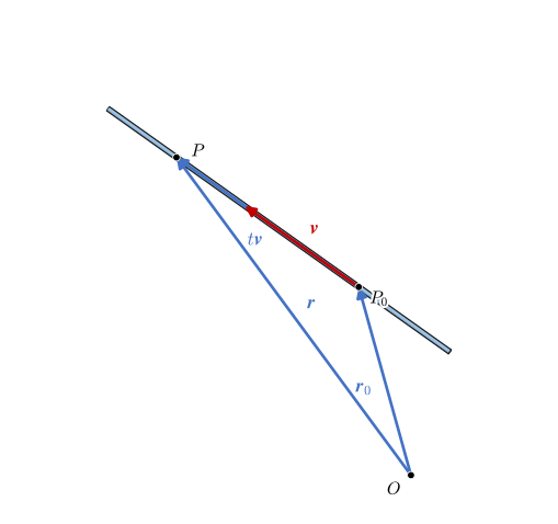
This is the line in vector form, also called parameter form. The line has no ends: letting the parameter \(t\) run through all real numbers gives all its points, negative \(t\) on the far side of \(P_0\), Figure 3.8.2. A step of \(t = 1\) is one length \(\lvert\bm v\rvert\), so \(t\) counts lengths only when \(\bm v\) is a unit vector.
In space a line has no single equation in \(x\), \(y\) and \(z\). It takes two, one for each of two planes that cross along it, while 3.8.1 does the job with one vector equation and also tells where on the line a point lies.
We model lines in vector form, \(\bm r = \bm r_0 + t\,\bm v\).
A line is most often fixed by two points \(P_1\) and \(P_2\). The vector between them lies along the line, so \(\bm r_0 = \bm r_1\) and \(\bm v = \bm r_2 - \bm r_1\) in 3.8.1, and collecting the terms of each point gives
\[ \boxed{\bm r = \bm r_1 + t\,(\bm r_2 - \bm r_1) = (1 - t)\,\bm r_1 + t\,\bm r_2} \tag{3.8.2}\]
The second form is a weighted average of the two points, with weights \(1 - t\) and \(t\) that add up to one, Figure 3.8.3. At \(t = 0\) all the weight sits on \(P_1\), at \(t = 1\) all of it on \(P_2\), and \(t = \tfrac12\) gives the midpoint. Values between 0 and 1 give the segment between the points. Outside that range one weight turns negative and the point is extrapolated along the rest of the line.
This is linear interpolation, and the parameter makes it a modelling tool. Nothing in 3.8.2 requires \(\bm r_1\) and \(\bm r_2\) to be positions. The same weights interpolate a temperature between two measurements, a value between two rows of a table, or a colour between two colours. When the parameter is a scaled time, \(t = \tau/T\) with \(\tau\) the time, the point travels from \(P_1\) to \(P_2\) in the time \(T\). A 3D printer or a CNC mill moves its tool this way, each straight move of its G-code interpolated between two end points, and the animations of this book move their points with the same formula. Curves traced in time return in Chapter 3.9.
Find the line through the points \(P_1 = (2, 4, -1)\) and \(P_2 = (5, 0, 7)\), and the points a quarter of the way and halfway from \(P_1\) to \(P_2\).
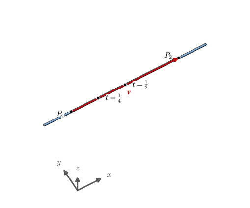
Either point serves as \(P_0\), and the vector from one point to the other lies along the line, Figure 3.8.4. With \(P_0 = P_1\),
\[ \bm r_0 = \bm r_{P_1} = \begin{bmatrix} 2 \\ 4 \\ -1 \end{bmatrix}, \qquad \bm v = \bm r_{P_2} - \bm r_{P_1} = \begin{bmatrix} 5 \\ 0 \\ 7 \end{bmatrix} - \begin{bmatrix} 2 \\ 4 \\ -1 \end{bmatrix} \]
and \(t = 1\) must land on \(P_2\). The two points sought are 3.8.2 at \(t = \tfrac14\) and \(t = \tfrac12\).
x, y, z, t = sp.symbols('x y z t', real=True)
rr_P1 = sp.Matrix([2, 4, -1])
rr_P2 = sp.Matrix([5, 0, 7])
rr_0 = rr_P1
vv = rr_P2 - rr_P1
rr = (1 - t)*rr_P1 + t*rr_P2 # the same line, as weights on the two pointsThe line and the two points are
\[ \begin{aligned}\bm r &= \left[\begin{matrix}2\\4\\-1\end{matrix}\right] + t\left[\begin{matrix}3\\-4\\8\end{matrix}\right],\quad \bm r(1) = \left[\begin{matrix}5\\0\\7\end{matrix}\right]\\ \bm r(\tfrac14) &= \left[\begin{matrix}\dfrac{11}{4}\\3\\1\end{matrix}\right],\quad \bm r(\tfrac12) = \left[\begin{matrix}\dfrac{7}{2}\\2\\3\end{matrix}\right]\end{aligned} \]
Another choice of point, \(P_2\), or of direction, \(-2\bm v\), describes the same line with another parameter.
Practise linear interpolation below, and the other constructions of the chapter after their examples. The Python switch turns each exercise into code: the same problem is solved with SymPy and checked when we run it.
Find the point \(P\) that lies 3 length units from \(P_0\), in the direction of \(\bm v\), on the line
\[ \bm r = \bm r_0 + t\,\bm v = \begin{bmatrix} 1 \\ 3 \\ 2 \end{bmatrix} + t\begin{bmatrix} -1 \\ 2 \\ 1 \end{bmatrix} \]
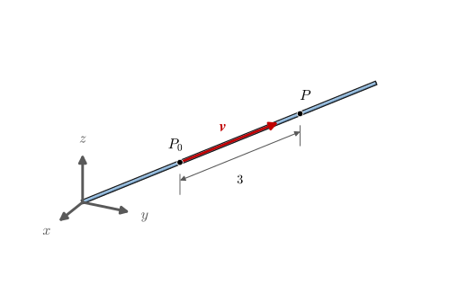
Three steps of \(\bm v\) would overshoot, since \(\lvert 3\bm v\rvert = 3\sqrt 6 > 3\). A distance is measured in steps of the unit vector \(\bm e_v = \bm v/\lvert\bm v\rvert\), which points the same way, so
\[ \bm r_P = \bm r_0 + 3\,\bm e_v = \bm r_0 + 3\,\frac{\bm v}{\lvert\bm v\rvert} \]
rr_0 = sp.Matrix([1, 3, 2])
vv = sp.Matrix([-1, 2, 1])

ee_v = vv/vv.norm()
rr_P = rr_0 + 3*ee_v
With \(\lvert\bm v\rvert = \sqrt 6\) we get
\[ \bm r_P = \left[\begin{matrix}1\\3\\2\end{matrix}\right] + 3\left[\begin{matrix}- \dfrac{\sqrt{6}}{6}\\\dfrac{\sqrt{6}}{3}\\\dfrac{\sqrt{6}}{6}\end{matrix}\right] = \left[\begin{matrix}1 - \dfrac{\sqrt{6}}{2}\\\sqrt{6} + 3\\\dfrac{\sqrt{6}}{2} + 2\end{matrix}\right]\approx\left[\begin{matrix}-0.2247\\5.449\\3.225\end{matrix}\right] \]
A distance between two objects is always the shortest one, and the shortest way from a point to a line is the perpendicular. Let \(\bm a\) be the vector from \(P_0\) to the point \(A\) and \(\bm d\) the vector from the line to \(A\) that is perpendicular to the line, Figure 3.8.7. Walking \(t\) steps along the line and then along \(\bm d\) reaches \(A\), so
\[ \begin{aligned} \bm a &= t\,\bm v + \bm d \\ \bm d \perp \bm v \;\Rightarrow\; \bm d\cdot\bm v &= 0 \end{aligned} \]
Inserting \(\bm d = \bm a - t\bm v\) in the second row gives \((\bm a - t\bm v)\cdot\bm v = 0\), and
\[ t = \frac{\bm a\cdot\bm v}{\bm v\cdot\bm v}, \qquad \bm d = \bm a - t\,\bm v \tag{3.8.3}\]
The vector \(t\bm v\) is the projection of \(\bm a\) on \(\bm v\) (Chapter 3.6), its shadow on the line, Figure 3.8.6.
The same \(t\) follows from asking for the shortest \(\bm d\) directly. Its squared length
\[ \lvert\bm d\rvert^2 = (\bm a - t\bm v)\cdot(\bm a - t\bm v) = \bm a\cdot\bm a - 2t\,\bm a\cdot\bm v + t^2\,\bm v\cdot\bm v \]
is a parabola in \(t\), least where its derivative \(-2\,\bm a\cdot\bm v + 2t\,\bm v\cdot\bm v\) is zero, and that gives 3.8.3 again. Perpendicular and shortest are the same condition. The derivative route needs no picture, so it carries over to problems with many distances at once.
Split the vector to the point into a part along the object and a part across it. The part across is the distance vector \(\bm d\), and its length is the distance.
Find the distance from the point \(A = (5, 4, -3)\) to the line
\[ L:\; \bm r = \begin{bmatrix} 1 \\ 3 \\ 2 \end{bmatrix} + t\begin{bmatrix} -1 \\ 2 \\ 1 \end{bmatrix} \]
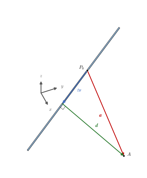
With \(\bm a = \bm r_A - \bm r_0\), 3.8.3 gives \(t\) and \(\bm d\), and the distance is
\[ d = \lvert\bm d\rvert = \lvert\bm a - t\,\bm v\rvert, \qquad t = \frac{\bm a\cdot\bm v}{\bm v\cdot\bm v} \]
The result must satisfy \(\bm d\cdot\bm v = 0\).
rr_0 = sp.Matrix([1, 3, 2])
vv = sp.Matrix([-1, 2, 1])
rr_A = sp.Matrix([5, 4, -3])

aa = rr_A - rr_0
t_A = aa.dot(vv)/vv.dot(vv)
dd = aa - t_A*vv
Projecting \(\bm a\) on the line gives
\[ \begin{aligned}\bm a &= \left[\begin{matrix}4\\1\\-5\end{matrix}\right],\quad t = \frac{\bm a\cdot\bm v}{\bm v\cdot\bm v} = - \dfrac{7}{6}\\ \bm d &= \bm a - t\bm v = \left[\begin{matrix}\dfrac{17}{6}\\\dfrac{10}{3}\\- \dfrac{23}{6}\end{matrix}\right],\quad \bm d\cdot\bm v = 0\\ d &= \lvert\bm d\rvert = \dfrac{\sqrt{1218}}{6}\approx5.817\end{aligned} \]
The vector \(\bm d\) tells us more than its length: it points from the line to \(A\), and it gives the foot of the perpendicular, \(\bm r_0 + t\bm v\).
Find the mirror point \(S\) of \(A\) in the line \(L\) of Example 3.
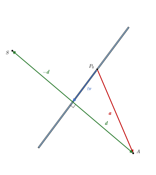
The mirror point lies as far from the line as \(A\), on the other side, Figure 3.8.8. Since \(\bm d\) was defined from the line to \(A\), we go from the foot of the perpendicular one \(\bm d\) the other way,
\[ \bm r_S = \bm r_0 + t\,\bm v - \bm d = \bm r_0 + \bm a - 2\bm d \]
The midpoint of \(A\) and \(S\) must be the foot, \(\tfrac12(\bm r_A + \bm r_S) = \bm r_0 + t\bm v\).
rr_S = rr_0 + t_A*vv - dd
rr_mid = (rr_A + rr_S)/2
Continuing from Example 3,
\[ \begin{aligned}\bm r_S &= \left[\begin{matrix}- \dfrac{2}{3}\\- \dfrac{8}{3}\\\dfrac{14}{3}\end{matrix}\right]\\ \tfrac12(\bm r_A + \bm r_S) &= \left[\begin{matrix}\dfrac{13}{6}\\\dfrac{2}{3}\\\dfrac{5}{6}\end{matrix}\right] = \left[\begin{matrix}\dfrac{13}{6}\\\dfrac{2}{3}\\\dfrac{5}{6}\end{matrix}\right]\end{aligned} \]
Two lines in space that neither meet nor are parallel are skew. Each has its own parameter, \(\bm r_1 = \bm r_{01} + s\,\bm v_1\) and \(\bm r_2 = \bm r_{02} + t\,\bm v_2\), and a pair \((s, t)\) picks one point on each line. The vector between them is
\[ \bm d = \bm r_2 - \bm r_1 \]
and it is shortest when it is perpendicular to both lines,
\[ \begin{aligned} \bm d\cdot\bm v_1 &= 0 \\ \bm d\cdot\bm v_2 &= 0 \end{aligned} \tag{3.8.4}\]
which are two linear equations for \(s\) and \(t\), Figure 3.8.9. Minimising \(\lvert\bm d\rvert^2\) over \(s\) and \(t\) gives the same pair, since \(\partial\lvert\bm d\rvert^2/\partial s = -2\,\bm d\cdot\bm v_1\) and \(\partial\lvert\bm d\rvert^2/\partial t = 2\,\bm d\cdot\bm v_2\). The two parameters must have different names: a shared \(t\) would tie the two points together and leave one unknown for two equations. Surveying and GPS positioning meet this problem, since two measured sight lines never meet exactly.
Find the distance between the lines
\[ L_1:\; \bm r_1 = \begin{bmatrix} 1 \\ 3 \\ 2 \end{bmatrix} + s\begin{bmatrix} -1 \\ 2 \\ 1 \end{bmatrix}, \qquad L_2:\; \bm r_2 = \begin{bmatrix} -1 \\ 1 \\ -3 \end{bmatrix} + t\begin{bmatrix} 1 \\ -3 \\ 2 \end{bmatrix} \]
and the two points where it occurs.
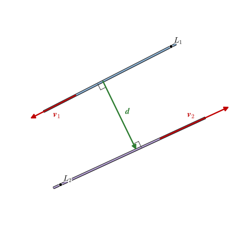
With \(\bm d = \bm r_2(t) - \bm r_1(s)\), 3.8.4 is
\[ \begin{aligned} \bigl(\bm r_{02} + t\bm v_2 - \bm r_{01} - s\bm v_1\bigr)\cdot\bm v_1 &= 0 \\ \bigl(\bm r_{02} + t\bm v_2 - \bm r_{01} - s\bm v_1\bigr)\cdot\bm v_2 &= 0 \end{aligned} \]
and SymPy solves the pair. Perpendicular to both lines means parallel to \(\bm v_1\times\bm v_2\) (Chapter 3.7), so the result must satisfy \(\bm d\times(\bm v_1\times\bm v_2) = \bm 0\).
s = sp.symbols('s', real=True)
vv_1, vv_2 = sp.Matrix([-1, 2, 1]), sp.Matrix([1, -3, 2])
rr_1 = sp.Matrix([1, 3, 2]) + s*vv_1
rr_2 = sp.Matrix([-1, 1, -3]) + t*vv_2

dd = rr_2 - rr_1
eqs = [sp.Eq(dd.dot(vv_1), 0), sp.Eq(dd.dot(vv_2), 0)]
sol = sp.solve(eqs, [s, t])

dd_min = dd.subs(sol)
check = dd_min.cross(vv_1.cross(vv_2))
The two perpendicularity conditions read
\[ \begin{aligned}\bm d\cdot\bm v_1 &= - 6 s - 5 t - 7 = 0 \\ \bm d\cdot\bm v_2 &= 5 s + 14 t - 6 = 0\end{aligned} \]
and their solution gives the shortest vector and its length,
\[ \begin{aligned}s &= - \dfrac{128}{59},\quad t = \dfrac{71}{59}\\ \bm d &= \left[\begin{matrix}- \dfrac{175}{59}\\- \dfrac{75}{59}\\- \dfrac{25}{59}\end{matrix}\right],\quad \bm d\times(\bm v_1\times\bm v_2) = \left[\begin{matrix}0\\0\\0\end{matrix}\right]\\ \lvert\bm d\rvert &= \dfrac{25 \sqrt{59}}{59}\approx3.255\end{aligned} \]
The two closest points are \(\bm r_1(s)\) and \(\bm r_2(t)\), and the point midway between them lies at the distance \(\tfrac12\lvert\bm d\rvert\) from both lines.
rr_1s, rr_2t = rr_1.subs(sol), rr_2.subs(sol)
rr_mid = (rr_1s + rr_2t)/2
Inserting \(s\) and \(t\),
\[ \begin{aligned}\bm r_1 &= \left[\begin{matrix}\dfrac{187}{59}\\- \dfrac{79}{59}\\- \dfrac{10}{59}\end{matrix}\right],\quad \bm r_2 = \left[\begin{matrix}\dfrac{12}{59}\\- \dfrac{154}{59}\\- \dfrac{35}{59}\end{matrix}\right]\\ \tfrac12(\bm r_1 + \bm r_2) &= \left[\begin{matrix}\dfrac{199}{118}\\- \dfrac{233}{118}\\- \dfrac{45}{118}\end{matrix}\right],\quad \tfrac12\lvert\bm d\rvert = \dfrac{25 \sqrt{59}}{118}\end{aligned} \]
Two measured sight lines toward the same target miss each other, and three lines have no point in common at all. When the measurements leave no exact answer, we choose the unknowns that make the sum of the squared distances least. This is the method of least squares, and the derivative route of the last two sections carries it out: write each squared distance in the unknowns, add them up, and set every partial derivative to zero. The squares keep the derivatives linear in the unknowns, so the conditions form a linear system.
For a point \(\bm p\) and several lines, each line \(i\) contributes \(\lvert\bm d_i\rvert^2\), with \(\bm d_i\) the distance vector from the line to \(\bm p\) of 3.8.3. Only the part of a move of \(\bm p\) across the line changes that distance, and the gradient of \(\lvert\bm d_i\rvert^2\) with respect to \(\bm p\) works out to \(2\bm d_i\). The best point therefore satisfies
\[ \sum_i \bm d_i = \bm 0 \tag{3.8.5}\]
so the distance vectors from the lines to the best point balance, Figure 3.8.11.
Three cameras at \(C_1 = (6, 0, 0)\), \(C_2 = (0, 6, 0)\) and \(C_3 = (0, 0, 5)\) see the same marker along the directions \(\bm v_1 = (-4, 2, 1)\), \(\bm v_2 = (2, -4, 1)\) and \(\bm v_3 = (2, 2, -3)\). Measurement errors make the three sight lines miss each other. Find the point \(\bm p\) that lies nearest to all three in the least-squares sense.
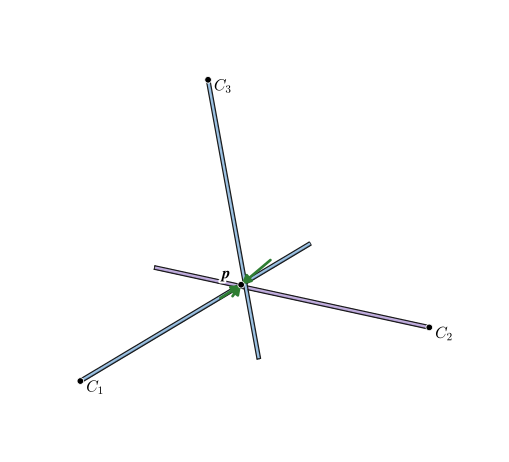
With \(\bm a_i = \bm p - \bm r_{C_i}\), 3.8.3 gives the distance vector from line \(i\) to \(\bm p\), and the sum of squares is
\[ \bm d_i = \bm a_i - \frac{\bm a_i\cdot\bm v_i}{\bm v_i\cdot\bm v_i}\,\bm v_i, \qquad D(x, y, z) = \lvert\bm d_1\rvert^2 + \lvert\bm d_2\rvert^2 + \lvert\bm d_3\rvert^2 \]
The conditions \(\partial D/\partial x = \partial D/\partial y = \partial D/\partial z = 0\) are three linear equations for the coordinates of \(\bm p\), Figure 3.8.12. The result must satisfy 3.8.5.
pp = sp.Matrix([x, y, z])
cameras = [sp.Matrix([6, 0, 0]), sp.Matrix([0, 6, 0]), sp.Matrix([0, 0, 5])]
sight = [sp.Matrix([-4, 2, 1]), sp.Matrix([2, -4, 1]), sp.Matrix([2, 2, -3])]

dds = []
for rr_C, vv in zip(cameras, sight):
    aa = pp - rr_C
    dds.append(aa - aa.dot(vv)/vv.dot(vv)*vv)     # what is left of a across the line

D = sum(dd.dot(dd) for dd in dds)
sol = sp.solve([D.diff(c) for c in (x, y, z)], [x, y, z])
pp_best = pp.subs(sol)
dds_best = [dd.subs(sol) for dd in dds]
Setting the three derivatives to zero gives the point, the three misses and the balance
\[ \begin{aligned}\bm p &= \left[\begin{matrix}\dfrac{244}{115}\\\dfrac{244}{115}\\\dfrac{53}{46}\end{matrix}\right]\approx\left[\begin{matrix}2.12\\2.12\\1.15\end{matrix}\right]\\ \lvert\bm d_1\rvert &\approx 0.229,\quad \lvert\bm d_2\rvert \approx 0.229,\quad \lvert\bm d_3\rvert \approx 0.456\\ \bm d_1 + \bm d_2 + \bm d_3 &= \left[\begin{matrix}0\\0\\0\end{matrix}\right]\end{aligned} \]
The third sight line passes twice as far from \(\bm p\) as the other two, which points to the third camera as the one to check first. A fourth camera adds a fourth term to \(D\), and the system stays three equations for the three coordinates.
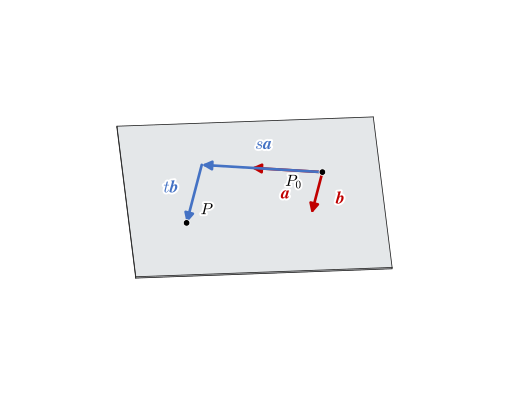
A plane is fixed by a point \(P_0\) in it, with position vector \(\bm r_0\), and two directions \(\bm a\) and \(\bm b\) along it that are not parallel. From \(P_0\) we reach any point of the plane by \(s\) steps of \(\bm a\) and \(t\) steps of \(\bm b\),
\[ \boxed{\bm r = \bm r_0 + s\,\bm a + t\,\bm b} \tag{3.8.6}\]
which is the plane in parameter form, Figure 3.8.13. The plane is two-dimensional, so it takes two parameters where the line took one, and the pair \((s, t)\) works as a coordinate system drawn on the plane.
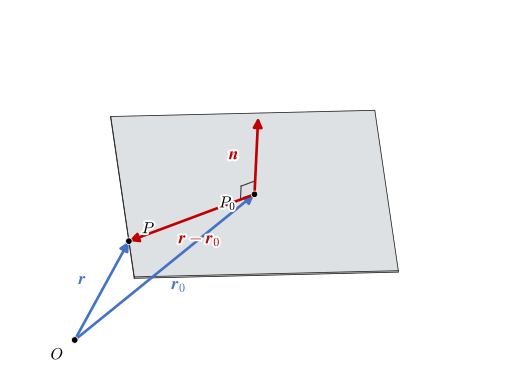
The normal \(\bm n = \bm a\times\bm b\) is perpendicular to both directions (Chapter 3.7) and therefore to every vector \(\bm r - \bm r_0\) from \(P_0\) to a point \(P\) in the plane, Figure 3.8.14. That gives the plane in vector form
\[ \boxed{(\bm r - \bm r_0)\cdot\bm n = 0} \tag{3.8.7}\]
Expanding the dot product gives the normal form, also called the affine form,
\[ \bigl((x, y, z) - (x_0, y_0, z_0)\bigr)\cdot(n_x, n_y, n_z) = 0 \quad\Longleftrightarrow\quad n_x x + n_y y + n_z z \underbrace{- (x_0 n_x + y_0 n_y + z_0 n_z)}_{\text{constant}} = 0 \]
The coefficients of \(x\), \(y\) and \(z\) in the normal form are the components of a normal vector. The planes we know first are the coordinate planes: the \(xy\), \(xz\) and \(yz\) planes all pass through the origin and have \(\bm k\), \(\bm j\) and \(\bm i\) as normals, so the \(xy\) plane is \(z = 0\).
Every pair \((s, t)\) in the parameter form gives a point, which is what we need to draw, mesh or interpolate a plane. The vector form answers the opposite question: \((\bm r - \bm r_0)\cdot\bm n\) is zero for a point in the plane, positive on the side \(\bm n\) points to and negative on the other. Examples 9 and 10 use that test.
The parameter form generates the points of a plane, and the vector form tests whether a point lies in it.
With three points \(P_1\), \(P_2\) and \(P_3\) of the plane, \(\bm a = \bm r_2 - \bm r_1\) and \(\bm b = \bm r_3 - \bm r_1\) turn the parameter form into linear interpolation between three points,
\[ \bm r = (1 - s - t)\,\bm r_1 + s\,\bm r_2 + t\,\bm r_3 \tag{3.8.8}\]
with three weights that add up to one, like the two of 3.8.2. All three weights are positive inside the triangle \(P_1P_2P_3\), and one of them turns negative outside it, so \(s \ge 0\), \(t \ge 0\), \(s + t \le 1\) is the triangle itself, Figure 3.8.15. Every surface in a CAD viewer, an STL file for 3D printing or a computer game is built from such triangles, and 3.8.8 interpolates positions, colours or temperatures over each of them.
A plane is given in normal form as \(-2y + 3z + 6 = 0\). Find its vector form.
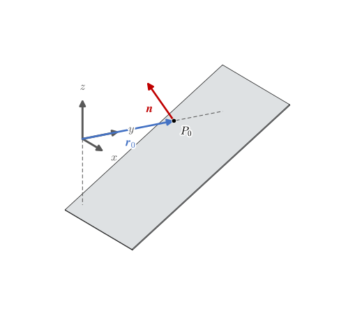
The normal is read off the coefficients, \(\bm n = (0, -2, 3)\). Any point of the plane serves as \(P_0\), and every plane crosses at least one coordinate axis. On an axis two of the coordinates are zero, so we try the three axes in turn,
\[ \begin{aligned} x\text{ axis}:\; (x_0, 0, 0) &: \quad -2\cdot 0 + 3\cdot 0 + 6 = 0 \\ y\text{ axis}:\; (0, y_0, 0) &: \quad -2 y_0 + 3\cdot 0 + 6 = 0 \end{aligned} \]
The first row reads \(6 = 0\) and has no solution, since the plane is parallel to the \(x\) axis. The second gives \(y_0 = 3\), Figure 3.8.16.
n_form = -2*y + 3*z + 6
nn = sp.Matrix([n_form.coeff(c) for c in (x, y, z)])     # the coefficients are the normal

on_x = sp.solve(n_form.subs({y: 0, z: 0}), x)           # empty: no crossing with the x axis
on_y = sp.solve(n_form.subs({x: 0, z: 0}), y)
rr_0 = sp.Matrix([0, on_y[0], 0])
plane = (sp.Matrix([x, y, z]) - rr_0).dot(nn)
The \(y\) axis gives the point, and the plane in vector form is
\[ \left(\left[\begin{matrix}x\\y\\z\end{matrix}\right] - \left[\begin{matrix}0\\3\\0\end{matrix}\right]\right)\cdot\left[\begin{matrix}0\\-2\\3\end{matrix}\right] = 0 \quad\Longleftrightarrow\quad - 2 y + 3 z + 6 = 0 \]
Find the plane through the points \(P_1 = (2, 4, -1)\), \(P_2 = (4, 3, 2)\) and \(P_3 = (5, 0, 7)\) in parameter form and in vector form, and check that the centroid of the triangle, at \(s = t = \tfrac13\), lies in the plane.
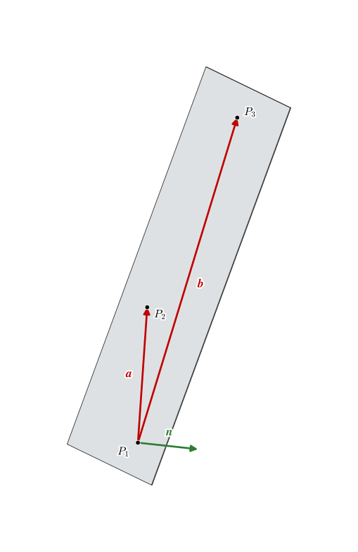
Three points fix a plane when they do not lie on one line. We take \(P_0 = P_1\) and form two vectors in the plane,
\[ \bm a = \bm r_{P_2} - \bm r_{P_1}, \qquad \bm b = \bm r_{P_3} - \bm r_{P_1} \]
which span the plane, Figure 3.8.17. A normal is perpendicular to both, and the cross product gives one (Chapter 3.7),
\[ \bm n = \bm a\times\bm b, \qquad (\bm r - \bm r_{P_1})\cdot\bm n = 0 \]
The other two points must satisfy the plane equation. The parameter form generates the centroid, \(\bm r_{P_1} + \tfrac13\bm a + \tfrac13\bm b\), and the vector form tests it.
rr_P1, rr_P2, rr_P3 = sp.Matrix([2, 4, -1]), sp.Matrix([4, 3, 2]), sp.Matrix([5, 0, 7])

aa = rr_P2 - rr_P1
bb = rr_P3 - rr_P1
nn = aa.cross(bb)
plane = sp.expand((sp.Matrix([x, y, z]) - rr_P1).dot(nn))
on_plane = [plane.subs(dict(zip((x, y, z), P))) for P in (rr_P2, rr_P3)]

rr_param = rr_P1 + s*aa + t*bb                            # generates the points
rr_G = rr_param.subs({s: sp.Rational(1, 3), t: sp.Rational(1, 3)})
G_test = plane.subs(dict(zip((x, y, z), rr_G)))           # tests one of them
The cross product gives the normal and the plane in both forms,
\[ \begin{aligned}\bm n &= \bm a\times\bm b = \left[\begin{matrix}2\\-1\\3\end{matrix}\right]\times\left[\begin{matrix}3\\-4\\8\end{matrix}\right] = \left[\begin{matrix}4\\-7\\-5\end{matrix}\right]\\ (\bm r - \bm r_{P_1})\cdot\bm n &= 4 x - 7 y - 5 z + 15 = 0\\ P_2,\, P_3 &: \quad 0,\;0\\ \bm r &= \left[\begin{matrix}2\\4\\-1\end{matrix}\right] + s\left[\begin{matrix}2\\-1\\3\end{matrix}\right] + t\left[\begin{matrix}3\\-4\\8\end{matrix}\right]\\ \bm r_G &= \left[\begin{matrix}\dfrac{11}{3}\\\dfrac{7}{3}\\\dfrac{8}{3}\end{matrix}\right],\quad (\bm r_G - \bm r_{P_1})\cdot\bm n = 0\end{aligned} \]
Had the three points been on one line, \(\bm a\) and \(\bm b\) would have been parallel and \(\bm a\times\bm b = \bm 0\).
The construction is the one for a point and a line, with the roles turned. Let \(\bm a\) be the vector from \(P_0\) to the point \(A\). The distance vector \(\bm d\) is perpendicular to the plane, so it lies along \(\bm n\) and is the projection of \(\bm a\) on \(\bm n\) (Chapter 3.6), Figure 3.8.18,
\[ \bm d = \frac{\bm a\cdot\bm n}{\bm n\cdot\bm n}\,\bm n, \qquad d = \lvert\bm d\rvert = \frac{\lvert\bm a\cdot\bm n\rvert}{\lvert\bm n\rvert} \tag{3.8.9}\]
The sign of \(\bm a\cdot\bm n\) tells the side: positive when \(A\) lies on the side \(\bm n\) points to.
Find the distance from the point \(A = (3, 2, -1)\) to the plane
\[ \left(\begin{bmatrix} x \\ y \\ z \end{bmatrix} - \begin{bmatrix} 2 \\ -1 \\ 3 \end{bmatrix}\right)\cdot\begin{bmatrix} 1 \\ -1 \\ 2 \end{bmatrix} = 0 \]
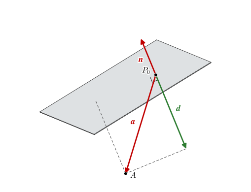
The plane gives \(\bm r_0 = (2, -1, 3)\) and \(\bm n = (1, -1, 2)\), and with \(\bm a = \bm r_A - \bm r_0\), 3.8.9 gives \(\bm d\), Figure 3.8.19.
rr_0 = sp.Matrix([2, -1, 3])
nn = sp.Matrix([1, -1, 2])
rr_A = sp.Matrix([3, 2, -1])

aa = rr_A - rr_0
dd = aa.dot(nn)/nn.dot(nn)*nn
Projecting \(\bm a\) on the normal gives
\[ \begin{aligned}\bm a &= \left[\begin{matrix}1\\3\\-4\end{matrix}\right],\quad \bm a\cdot\bm n = -10,\quad \bm n\cdot\bm n = 6\\ \bm d &= \left[\begin{matrix}- \dfrac{5}{3}\\\dfrac{5}{3}\\- \dfrac{10}{3}\end{matrix}\right]\\ d &= \lvert\bm d\rvert = \dfrac{5 \sqrt{6}}{3}\approx4.082\end{aligned} \]
The negative \(\bm a\cdot\bm n\) places \(A\) on the side of the plane away from \(\bm n\).
Find the intersection point \(Q\) of the line \(\bm r = (1, 3, 2) + t(-1, 2, 1)\) and the plane of Example 3.8.
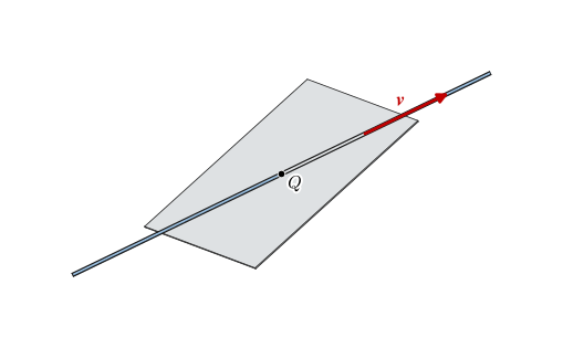
The point \(Q\) lies both on the line and in the plane, so the line’s \(\bm r\) satisfies the plane equation. With \(\bm r_{P_0} = (2, -1, 3)\) the point of the plane, inserting the line gives one equation for \(t\),
\[ \bigl(\bm r_0 + t\,\bm v - \bm r_{P_0}\bigr)\cdot\bm n = 0 \quad\Rightarrow\quad t = \frac{(\bm r_{P_0} - \bm r_0)\cdot\bm n}{\bm v\cdot\bm n} \]
The line enters in parameter form and the plane in vector form: one generates the candidate points, the other tests them. The parameter tells how many steps of \(\bm v\) lead from \(\bm r_0\) to the plane, Figure 3.8.21. If \(\bm v\cdot\bm n = 0\) the line runs parallel to the plane: it either lies in it or never meets it.
rr_0, vv = sp.Matrix([1, 3, 2]), sp.Matrix([-1, 2, 1])
rr_P0, nn = sp.Matrix([2, -1, 3]), sp.Matrix([1, -1, 2])

line = rr_0 + t*vv
t_Q = sp.solve((line - rr_P0).dot(nn), t)[0]
rr_Q = line.subs(t, t_Q)
Inserting the line in the plane equation gives
\[ \begin{aligned}(\bm r_0 + t\bm v - \bm r_{P_0})\cdot\bm n &= - t - 7 = 0 \quad\Rightarrow\quad t = -7\\ \bm r_Q &= \left[\begin{matrix}8\\-11\\-5\end{matrix}\right]\end{aligned} \]
The line meets the plane at \(Q = (8, -11, -5)\). Since \(\bm v\cdot\bm n = -1\) is small against \(\lvert\bm v\rvert\lvert\bm n\rvert = 6\), the line crosses the plane at a shallow angle, which is why the intersection lies seven steps from \(\bm r_0\).
A probe that measures the height of a machined surface at a few points returns points that lie near a plane without lying in it, and the least-squares plane is the reference the deviations are judged against. With the plane written as \(z = c_0 + c_1 x + c_2 y\), the measured height \(z_i\) above the point \((x_i, y_i)\) misses the plane by the residual
\[ e_i = z_i - (c_0 + c_1 x_i + c_2 y_i) \]
and minimising \(\sum e_i^2\) gives three linear equations for \(c_0\), \(c_1\) and \(c_2\). Moving \(c_1 x + c_2 y\) to the left side gives the normal form \(-c_1 x - c_2 y + z - c_0 = 0\), so the normal \(\bm n = (-c_1, -c_2, 1)\) is read off as in Example 7. The derivative with respect to \(c_0\) is \(-2\sum e_i\), so the residuals of the fit add up to zero.
The residual \(e_i\) is measured vertically. The distance from the point to the plane is \(e_i\,n_z/\lvert\bm n\rvert\) by 3.8.9, and for a nearly horizontal plane the factor is close to one and the two agree. Fitting the perpendicular distances themselves leads to an eigenvalue problem, which returns with the matrices.
A probe measures the height \(z\) of a plate at six points of a grid, all in millimetres.
| \(x\) | 0 | 200 | 400 | 0 | 200 | 400 |
|---|---|---|---|---|---|---|
| \(y\) | 0 | 0 | 0 | 300 | 300 | 300 |
| \(z\) | 0.10 | 0.22 | 0.31 | 0.43 | 0.48 | 0.62 |
Find the least-squares plane, its normal, and the flatness of the plate, the spread between the largest and the smallest residual.
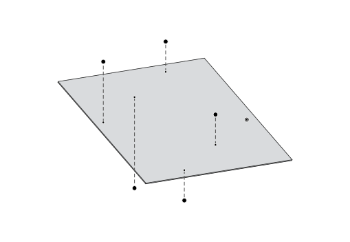
The residuals are linear in \(c_0\), \(c_1\) and \(c_2\), so SymPy solves \(\partial\sum e_i^2/\partial c_k = 0\) for the three coefficients, Figure 3.8.22. The residuals of the fit must add up to zero.
c_0, c_1, c_2 = sp.symbols('c_0 c_1 c_2', real=True)
xs = [0, 200, 400, 0, 200, 400]
ys = [0, 0, 0, 300, 300, 300]
zs = [sp.Rational(h) for h in ('0.10', '0.22', '0.31', '0.43', '0.48', '0.62')]

ee = [z_i - (c_0 + c_1*x_i + c_2*y_i) for x_i, y_i, z_i in zip(xs, ys, zs)]
E = sum(e**2 for e in ee)
sol = sp.solve([E.diff(c) for c in (c_0, c_1, c_2)], [c_0, c_1, c_2])

ee_fit = [e.subs(sol) for e in ee]
nn = sp.Matrix([-sol[c_1], -sol[c_2], 1])          # from -c1 x - c2 y + z - c0 = 0
flatness = max(ee_fit) - min(ee_fit)
The fit gives the plane, its normal and the residuals, in millimetres,
\[ \begin{aligned}z &= 0.0005 x + 0.001 y + 0.11,\quad \bm n = \left[\begin{matrix}-0.0005\\-0.001\\1.0\end{matrix}\right]\\ e_i &= \left[\begin{matrix}-0.01 & 0.01 & 0 & 0.02 & -0.03 & 0.01\end{matrix}\right],\quad \textstyle\sum e_i = 0\\ \text{flatness} &= e_{\max} - e_{\min} = 0.05\ \text{mm}\end{aligned} \]
Over 400 mm the plane rises 0.2 mm, so \(n_z/\lvert\bm n\rvert\) differs from one by less than \(10^{-6}\) and the vertical residuals are the distances to the plane. The plate is flat to within 0.05 mm.