“It will be convenient to introduce here a notion (which plays a conspicuous part in my new theory of multiple algebra), namely that of the latent roots of a matrix—latent in a somewhat similar sense as vapour may be said to be latent in water or smoke in a tobacco-leaf.”
— James Joseph Sylvester, On the equation to the secular inequalities in the planetary theory, 1883
A square matrix \(\bm A\) turns most vectors into vectors that point in a new direction. Along a few directions the map only stretches, shrinks or reverses. A non-zero vector \(\bm x\) along such a direction is an eigenvector of \(\bm A\), and the factor \(\lambda\) it is scaled by is the eigenvalue that belongs to it,
\[
\boxed{\bm A\bm x = \lambda\bm x, \qquad \bm x \ne \bm 0}
\tag{3.14.1}\]
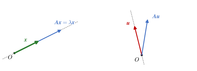
In the words of the vector chapters, \(\bm A\bm x\) is parallel to \(\bm x\), Figure 3.14.1. A value \(\lambda > 1\) stretches the vector, \(0 < \lambda < 1\) shrinks it, a negative \(\lambda\) turns it around, and \(\lambda = 0\) sends the whole line to the origin. The zero vector is left out of the definition, since \(\bm A\bm 0 = \lambda\bm 0\) holds for every \(\lambda\) and tells us nothing. Sylvester’s latent roots are the eigenvalues; the German eigen, own, is the name that stuck.
Figure 3.14.1: Left: the eigenvector \(\bm x\) and its image \(\bm A\bm x = \lambda\bm x\) lie on one line through \(O\). Right: a vector \(\bm u\) that the map turns off its line.
Directions that stay on their line
The video plays the map of Example 1 below on a fan of unit vectors. Every vector turns away from its own line except those on the two green lines. Along one of them the vectors keep their length, \(\lambda_1 = 1\); along the other they grow four times, \(\lambda_2 = 4\).
Two consequences of 3.14.1 follow from the rules of the matrix product (Chapter 3.10). If \(\bm x\) is an eigenvector, so is every multiple \(s\bm x\) with \(s\ne 0\), since
\[
\bm A(s\bm x) = s\bm A\bm x = s\lambda\bm x = \lambda(s\bm x)
\]
and if \(\bm x_1\) and \(\bm x_2\) are eigenvectors for the same \(\lambda\), so is their sum, since \(\bm A(\bm x_1 + \bm x_2) = \lambda\bm x_1 + \lambda\bm x_2 = \lambda(\bm x_1 + \bm x_2)\). An eigenvector therefore stands for a whole line through the origin.
An eigenvector is fixed only up to a factor. We pick small integers, or divide by the length to get a unit vector.
Not every map has such a line. A rotation of the plane by \(90^\circ\) turns every vector off its line, so no real \(\lambda\) satisfies 3.14.1; its eigenvalues are complex numbers, which we leave aside.
Grant Sanderson’s video below shows the same idea with the span of each vector, and adds the rotation in space, whose eigenvector is its axis.
The characteristic equation
Moving \(\lambda\bm x\) to the left side of 3.14.1 and writing \(\lambda\bm x = \lambda\bm I\bm x\), so that both terms carry a matrix, gives
\[
(\bm A - \lambda\bm I)\,\bm x = \bm 0
\tag{3.14.2}\]
a homogeneous linear system (Chapter 3.12). It always has the solution \(\bm x = \bm 0\). A non-zero solution exists only when \(\bm A - \lambda\bm I\) crushes some direction onto the origin, that is, when the matrix is singular and its determinant vanishes (Chapter 3.11),
\[
\boxed{\det(\bm A - \lambda\bm I) = 0}
\tag{3.14.3}\]
This is the characteristic equation of \(\bm A\). For a \(2\times 2\) matrix it reads
and for an \(n\times n\) matrix the determinant is a polynomial of degree \(n\) in \(\lambda\), which has \(n\) roots when they are counted with multiplicity. Each real root is an eigenvalue. The eigenvectors that belong to it are the non-zero solutions of 3.14.2 with that \(\lambda\) inserted, the null space of \(\bm A - \lambda\bm I\).
In the video \(\lambda\) runs from 0 to 5 and the plane is drawn under \(\bm A - \lambda\bm I\), with \(\bm A\) from Example 1. The image of the unit square, whose signed area is \(\det(\bm A - \lambda\bm I)\), collapses onto a segment at \(\lambda = 1\) and again at \(\lambda = 4\). At each of these values one eigenvector is crushed to the origin, and the determinant, drawn on the right as a function of \(\lambda\), passes through zero.
Expand \(\det(\bm A - \lambda\bm I)\) and solve the characteristic equation for the eigenvalues \(\lambda_k\).
For each \(\lambda_k\), write out the rows of \((\bm A - \lambda_k\bm I)\bm x = \bm 0\). They are linearly dependent, so for a \(2\times 2\) matrix one row fixes the direction of \(\bm x_k\).
Check that \(\bm A\bm x_k = \lambda_k\bm x_k\).
If the rows in step 2 are not parallel, the eigenvalue is wrong: only a singular matrix leaves a line of solutions.
Example 1: Eigenvalues and eigenvectors of a 2×2 matrix
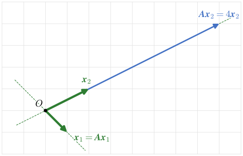
Figure 3.14.2: The eigenvectors of \(\bm A\): \(\bm x_1 = (1, -1)\) is left as it is, \(\bm x_2 = (2, 1)\) is stretched four times. The dashed lines are the two eigen-directions.
with the roots \(\lambda_1 = 1\) and \(\lambda_2 = 4\). For \(\lambda_1 = 1\) the two rows of \((\bm A - \bm I)\bm x = \bm 0\) are
\[
\begin{aligned}
2x + 2y &= 0 \\
x + y &= 0
\end{aligned}
\]
which say the same thing, as they must. Choosing \(x = 1\) gives \(y = -1\) and \(\bm x_1 = (1, -1)^\mathsf{T}\). For \(\lambda_2 = 4\) the rows are \(-x + 2y = 0\) and \(x - 2y = 0\), and \(x = 2\) gives \(\bm x_2 = (2, 1)^\mathsf{T}\). The check \(\bm A\bm x_2 = (3\cdot 2 + 2\cdot 1,\ 1\cdot 2 + 2\cdot 1)^\mathsf{T} = (8, 4)^\mathsf{T} = 4\bm x_2\) holds, Figure 3.14.2.
SymPy follows the procedure step by step: the determinant, its roots, and the null space of \(\bm A - \lambda\bm I\) for each root.
Code
AA = sp.Matrix([[3, 2], [1, 2]])lam = sp.symbols('lambda', real=True)char = (AA - lam*sp.eye(2)).det()lams = sp.solve(char, lam)# the eigenvectors are the null space of A - lambda I, one line for each rootxx_1 = (AA - lams[0]*sp.eye(2)).nullspace()[0]xx_2 = (AA - lams[1]*sp.eye(2)).nullspace()[0]
The characteristic polynomial, its roots and the two eigenvectors are
SymPy scales the null-space vector so that its last component is one, so \(\bm x_2 = (2, 1)^\mathsf{T}\) appears as we chose it and \(\bm x_1\) appears as \((-1, 1)^\mathsf{T}\), the same line traversed the other way. The method AA.eigenvects() does all of it at once and returns, for each eigenvalue, the eigenvalue, its multiplicity as a root and a list of eigenvectors. The check \(\bm A\bm x_k - \lambda_k\bm x_k = \bm 0\) closes the example.
Code
eig = AA.eigenvects() # [(lambda, multiplicity, [x, ...]), ...]checks = [AA*xx - l*xx for l, m, (xx,) in eig]
For both eigenpairs the check gives the zero vector,
NumPy computes eigenvalues with floating-point numbers. np.linalg.eig returns the eigenvalues and a matrix whose columns are the eigenvectors, each scaled to unit length, in an order and with signs of its own choosing. Since a real matrix may have complex eigenvalues, the result can come back as complex numbers with zero imaginary parts, which .real removes.
Code
A = np.array([[3.0, 2.0], [1.0, 2.0]])res = np.linalg.eig(A) # column k of the eigenvectors belongs to eigenvalue klam_np, X_np = res.eigenvalues.real, res.eigenvectors.real # drop the zero imaginary parts
The eigenvalues and the matrix of unit eigenvectors are
NumPy lists \(\lambda = 4\) first. Its first column is \((2, 1)^\mathsf{T}/\sqrt 5 \approx (0.894, 0.447)^\mathsf{T}\), our \(\bm x_2\) divided by its length, and its second column is \((-1, 1)^\mathsf{T}/\sqrt 2\), the line of \(\bm x_1\). Code that uses the result must therefore pair each column with its own eigenvalue and never rely on the order.
Practise the eigenvalues of a \(2\times 2\) matrix below. The answer sheet also shows the shortcut of the section A shortcut for 2×2 matrices, which we meet later in the chapter.
Practise eigenvectors below: the eigenvalue is given, and any non-zero multiple of the eigenvector counts as right.
Symmetric matrices
A symmetric matrix, \(\bm A^\mathsf{T} = \bm A\), has eigenvalues and eigenvectors with two properties that the rest of the book relies on.
The eigenvalues are real. For a \(2\times 2\) symmetric matrix with entries \(a\), \(b\), \(b\), \(d\) the characteristic equation 3.14.4 is \(\lambda^2 - (a + d)\lambda + ad - b^2 = 0\), whose discriminant
\[
(a + d)^2 - 4(ad - b^2) = (a - d)^2 + 4b^2 \ge 0
\]
is a sum of squares and never negative. The same holds for symmetric matrices of any size, although the proof needs complex numbers.
Eigenvectors of different eigenvalues are perpendicular. Let \(\bm A\bm x_1 = \lambda_1\bm x_1\) and \(\bm A\bm x_2 = \lambda_2\bm x_2\). Multiplying the first equation by \(\bm x_2^\mathsf{T}\) from the left gives the number \(\bm x_2^\mathsf{T}\bm A\bm x_1 = \lambda_1\,\bm x_2^\mathsf{T}\bm x_1\). A number is its own transpose, and with \((\bm A\bm B)^\mathsf{T} = \bm B^\mathsf{T}\bm A^\mathsf{T}\) from Chapter 3.10 and \(\bm A^\mathsf{T} = \bm A\),
Both \(\bm x_2^\mathsf{T}\bm x_1\) and \(\bm x_1^\mathsf{T}\bm x_2\) are the dot product \(\bm x_1\cdot\bm x_2\) (Chapter 3.6), so the two expressions together give
and when \(\lambda_1 \ne \lambda_2\) the dot product must vanish.
A symmetric matrix has real eigenvalues, and eigenvectors of different eigenvalues are orthogonal.
The video plays the symmetric matrix of Example 2 on the unit circle. The circle becomes an ellipse whose axes lie along the two perpendicular eigen-directions, with the half-axes \(|\lambda_1|\) and \(|\lambda_2|\). The stress and strain at a point are symmetric matrices of this kind: their eigenvalues are the principal stresses and strains and their eigenvectors the principal directions, Chapter 8.7, and Chapter 8.8 draws the \(2\times 2\) case as a circle.
Example 2: A symmetric matrix
Find the eigenvalues and eigenvectors of the symmetric matrix
and check that the eigenvectors are perpendicular.
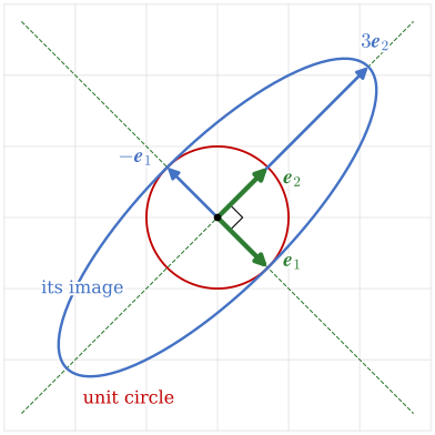
Figure 3.14.3: The unit circle and its image under \(\bm B\), an ellipse with its axes along the unit eigenvectors \(\bm e_1\) and \(\bm e_2\). Along \(\bm e_1\) the map reverses, \(\lambda_1 = -1\); along \(\bm e_2\) it stretches three times.
The characteristic equation is \((1 - \lambda)^2 - 4 = \lambda^2 - 2\lambda - 3 = 0\) with the roots \(\lambda_1 = -1\) and \(\lambda_2 = 3\). For \(\lambda_1 = -1\) the first row of 3.14.2 reads \(2x + 2y = 0\), which gives \(\bm x_1 = (1, -1)^\mathsf{T}\), and for \(\lambda_2 = 3\) it reads \(-2x + 2y = 0\), which gives \(\bm x_2 = (1, 1)^\mathsf{T}\). The dot product \(\bm x_1\cdot\bm x_2 = 1 - 1 = 0\) confirms the right angle. Divided by their lengths, the eigenvectors become the unit vectors \(\bm e_1\) and \(\bm e_2\) of Figure 3.14.3.
For symmetric matrices NumPy has np.linalg.eigh, which returns the eigenvalues in ascending order and orthonormal eigenvectors as columns. Collected as the columns of a matrix \(\bm Q = [\bm e_1\ \bm e_2]\), they satisfy \(\bm Q^\mathsf{T}\bm Q = \bm I\): \(\bm Q\) is orthogonal (Chapter 3.11).
The negative eigenvalue reverses the vectors along \(\bm x_1\). The ellipse in Figure 3.14.3 does not show the reversal, since a reversed ellipse is the same ellipse; the arrows of \(\bm e_1\) and its image \(-\bm e_1\) do.
Practise symmetric matrices below. The unit eigenvector may point either way along its line.
Diagonalisation
The two equations \(\bm A\bm x_1 = \lambda_1\bm x_1\) and \(\bm A\bm x_2 = \lambda_2\bm x_2\) can be written side by side. With the eigenvectors as the columns of \(\bm P = [\bm x_1\ \bm x_2]\) and the eigenvalues on the diagonal of \(\bm D\), column \(k\) of \(\bm A\bm P\) is \(\bm A\bm x_k\), and column \(k\) of \(\bm P\bm D\) is \(\lambda_k\bm x_k\),
When the eigenvectors are linearly independent, \(\bm P\) has an inverse, and multiplying by \(\bm P^{-1}\) from the right gives
\[
\boxed{\bm A = \bm P\bm D\bm P^{-1}}
\tag{3.14.5}\]
Read from right to left, 3.14.5 is three maps in sequence. \(\bm P^{-1}\) takes a vector to its components in the basis of eigenvectors, which carries \(\bm x_1\) to \(\bm i\) and \(\bm x_2\) to \(\bm j\); \(\bm D\) scales each component by its own eigenvalue; and \(\bm P\) takes the result back to the standard basis. This is the change of basis of Chapter 3.13: in the eigenvector basis, the matrix of the map is diagonal, \(\bm P^{-1}\bm A\bm P = \bm D\). The video plays the three maps for Example 1 and ends where \(\bm A\) ends.
For a symmetric matrix the unit eigenvectors are orthonormal, so \(\bm P\) is an orthogonal matrix \(\bm Q\) with \(\bm Q^{-1} = \bm Q^\mathsf{T}\), and
\[
\bm A = \bm Q\bm D\bm Q^\mathsf{T}
\tag{3.14.6}\]
The map is then a rotation (or reflection) to the eigen-axes, a scaling along each axis, and the rotation back.
Diagonalisation makes powers cheap. In \(\bm A^n = \bm P\bm D\bm P^{-1}\,\bm P\bm D\bm P^{-1}\cdots\bm P\bm D\bm P^{-1}\) every inner \(\bm P^{-1}\bm P\) is \(\bm I\), so
The same follows for a single vector. Writing \(\bm x_0 = c_1\bm x_1 + c_2\bm x_2\) in the eigenvector basis, each application of \(\bm A\) multiplies each term by its eigenvalue,
so the eigenvalues decide what repeated maps do: a term with \(|\lambda| < 1\) dies out, a term with \(|\lambda| > 1\) grows without bound, and a term with \(\lambda = 1\) stays. The same argument gives the eigenvalues \(\lambda^n\) for \(\bm A^n\) and \(1/\lambda\) for \(\bm A^{-1}\), since \(\bm A\bm x = \lambda\bm x\) gives \(\bm x = \lambda\bm A^{-1}\bm x\). A matrix is singular exactly when \(\lambda = 0\) is one of its eigenvalues, because then \(\det(\bm A - 0\,\bm I) = \det\bm A = 0\).
Not every matrix can be diagonalised. The shear \(\begin{bmatrix} 1 & 1 \\ 0 & 1 \end{bmatrix}\) has the double eigenvalue \(\lambda = 1\) but only one eigen-direction, the \(x\) axis, so there is no second column for \(\bm P\). Symmetric matrices can always be diagonalised.
Example 3: Powers of a matrix
Find \(\bm A^n\) in closed form for the matrix \(\bm A\) of Example 1, Figure 3.14.2, and check the result for \(n = 3\).
With the eigenvectors of Example 1 as columns and the eigenvalues on the diagonal,
For \(n = 1\) the result is \(\frac13\begin{bmatrix} 9 & 6 \\ 3 & 6 \end{bmatrix} = \bm A\), as it must be. SymPy’s AA.diagonalize() returns \(\bm P\) and \(\bm D\); its columns may come in another order or scaled differently, which leaves \(\bm P\bm D^n\bm P^{-1}\) unchanged.
Code
n = sp.symbols('n', integer=True, nonnegative=True)AA = sp.Matrix([[3, 2], [1, 2]])PP, DD = AA.diagonalize()DD_n = sp.diag(*[DD[k, k]**n for k inrange(2)]) # a diagonal matrix: power each entryAA_n = PP*DD_n*PP.inv()AA_n3 = (3*AA_n).applyfunc(sp.expand) # shown as one third of an integer patterncheck = AA_n.subs(n, 3) - AA**3
The diagonalisation, the closed form and the check against \(\bm A^3\) computed directly are
The entries grow as \(4^n\), the larger eigenvalue, and for large \(n\) the columns of \(\bm A^n\) both point along \(\bm x_2 = (2, 1)^\mathsf{T}\): repeated maps turn every vector toward the eigen-direction with the largest \(|\lambda|\).
Practise 3.14.8 below: write the start vector in the eigenvector basis, then raise the eigenvalues to the power.
Example 4: Grass and bushes on a meadow
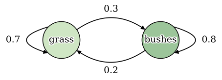
A meadow left to itself holds only grass and bushes. In one growing season bushes take over 30 % of the land that was grass, and 20 % of the bushes die and the land returns to grass, Figure 3.14.4. Ten percent of the meadow is covered by bushes at the start. After how many seasons is half the meadow covered by bushes, and is there a steady state?
Figure 3.14.4: The shares of land that move between grass and bushes in one season.
Let \(x_g\) and \(x_b\) be the shares of grass and bushes, with \(x_g + x_b = 1\), and \(\bm x_n = (x_g, x_b)^\mathsf{T}\) the state after \(n\) seasons. The two observations give the state one season later,
The matrix \(\bm T\) is a transition matrix: column \(k\) tells where the land of type \(k\) goes, and each column adds up to one, so no land is lost. Starting from \(\bm x_0 = (0.9, 0.1)^\mathsf{T}\), the state after \(n\) seasons is \(\bm x_n = \bm T^n\bm x_0\).
The characteristic equation \((0.7 - \lambda)(0.8 - \lambda) - 0.06 = \lambda^2 - 1.5\lambda + 0.5 = 0\) has the roots \(\lambda_1 = 1\) and \(\lambda_2 = \tfrac12\), with the eigenvectors \(\bm x_1 = (2, 3)^\mathsf{T}\) from \(-0.3x + 0.2y = 0\) and \(\bm x_2 = (-1, 1)^\mathsf{T}\) from \(0.2x + 0.2y = 0\). Writing \(\bm x_0 = c_1\bm x_1 + c_2\bm x_2\) gives \(c_1 = \tfrac15\) and \(c_2 = -\tfrac12\), and by 3.14.8
The first term is the eigenvector of \(\lambda_1 = 1\), scaled so that its components add up to one; the second halves every season. The share of bushes reaches one half when \(0.6 - (\tfrac12)^{n+1} = 0.5\), that is, when \(2^{n+1} = 10\).
Code
TT = sp.Matrix([[sp.Rational(7, 10), sp.Rational(2, 10)], [sp.Rational(3, 10), sp.Rational(8, 10)]])xx_0 = sp.Matrix([sp.Rational(9, 10), sp.Rational(1, 10)])states = [TT**k*xx_0 for k inrange(5)] # season by season(l_2, _, (xx_2,)), (l_1, _, (xx_1,)) = TT.eigenvects() # ascending: 1/2, then 1cc = sp.Matrix.hstack(xx_1, xx_2).solve(xx_0) # x0 in the eigenvector basisxx_n = cc[0]*l_1**n*xx_1 + cc[1]*l_2**n*xx_2n_half = sp.solve(sp.Eq(xx_n[1], sp.Rational(1, 2)), n)
The first four seasons, computed by repeated multiplication, are
SymPy scales \(\bm x_1\) to \((2/3, 1)^\mathsf{T}\), so its \(c_1 = 3/5\) differs from ours, but the product \(c_1\bm x_1 = (0.4, 0.6)^\mathsf{T}\) is the same. Half the meadow is covered by bushes during the third season, at \(n \approx 2.3\), and the table confirms it: \(x_b\) is 0.475 after two seasons and 0.5375 after three. The state then settles at 40 % grass and 60 % bushes.
The steady state does not depend on the start. Any start whose shares add up to one has the same \(c_1\), since the components of \(c_2\bm x_2\) add up to zero, and the \(\lambda_2\) term dies out. A system \(\bm x_{n+1} = \bm T\bm x_n\) of this kind is a discrete dynamical system. It settles when one eigenvalue is 1 and all others satisfy \(|\lambda| < 1\), and its steady state is the eigenvector of \(\lambda = 1\). The video iterates the meadow season by season; the remainder \(c_2(\tfrac12)^n\bm x_2\), drawn in orange, halves along the line \(x_g + x_b = 1\) while the whole square of states shrinks onto the eigen-direction of \(\lambda = 1\).
Practise the steady state of a two-state transition matrix below. The dots are the states season by season from all land in state 1.
A shortcut for 2×2 matrices
A quadratic with the roots \(\lambda_1\) and \(\lambda_2\) factors as \((\lambda - \lambda_1)(\lambda - \lambda_2) = \lambda^2 - (\lambda_1 + \lambda_2)\lambda + \lambda_1\lambda_2\). Comparing with 3.14.4 term by term,
\[
\lambda_1 + \lambda_2 = a_{11} + a_{22} = \operatorname{tr}\bm A, \qquad \lambda_1\lambda_2 = \det\bm A
\tag{3.14.9}\]
The eigenvalues add up to the trace (Chapter 3.10) and multiply to the determinant; the same holds for the \(n\) eigenvalues of an \(n\times n\) matrix. For a \(2\times 2\) matrix the two eigenvalues lie symmetrically about their mean \(m = \tfrac12\operatorname{tr}\bm A\), at the distance that makes their product \(p = \det\bm A\),
\[
\boxed{\lambda = m \pm \sqrt{m^2 - p}, \qquad m = \tfrac12\operatorname{tr}\bm A, \quad p = \det\bm A}
\tag{3.14.10}\]
For Example 1, \(m = \tfrac52\) and \(p = 4\) give \(\lambda = \tfrac52 \pm \tfrac32\), that is 1 and 4. For the meadow, \(m = \tfrac34\) and \(p = 0.56 - 0.06 = 0.5\) give \(\tfrac34 \pm \tfrac14\), that is 1 and \(\tfrac12\). For the rotation by the angle \(\theta\), \(m = \cos\theta\) and \(p = 1\), so \(m^2 - p = -\sin^2\theta\) is negative for every angle except \(0\) and \(\pi\): the eigenvalues are complex and no direction stays on its line, as we saw for the quarter turn. Grant Sanderson derives the shortcut in the video below.
NoteWhere the eigenvalues lie
Each eigenvalue of an \(n\times n\) matrix lies within the distance \(r_i = \sum_{j\ne i}|a_{ij}|\) of at least one diagonal entry \(a_{ii}\), a theorem published by Semyon Gershgorin in 1931. For
the three discs are \(|\lambda - 2| \le 4\), \(|\lambda + 4| \le 8\) and \(|\lambda - 7| \le 13\). The characteristic equation \(\lambda^3 - 5\lambda^2 - 76\lambda + 80 = (\lambda - 1)(\lambda^2 - 4\lambda - 80) = 0\) gives \(\lambda = 1\) and \(\lambda = 2 \pm 2\sqrt{21}\), that is \(11.17\) and \(-7.17\), and each lies in at least one disc. In general the discs lie in the complex plane, since the eigenvalues may be complex. The theorem costs a few additions and gives a quick check on eigenvalues computed by a program.
Fitting a plane with perpendicular distances
Chapter 3.8 fitted a plane \(z = c_0 + c_1x + c_2y\) to measured points by making the sum of the squared vertical residuals least. The distance from a point to a plane is measured along the normal, and fitting these perpendicular distances leads to an eigenvalue problem.
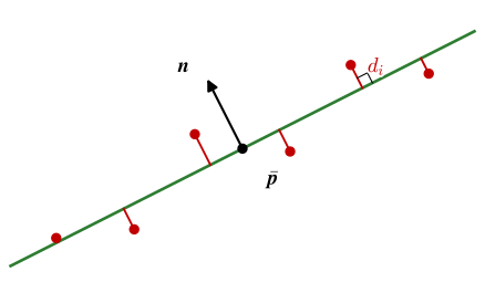
Figure 3.14.5: A section through the points: the best plane passes through the centroid \(\bar{\bm p}\), and its unit normal \(\bm n\) makes the perpendicular distances \(d_i\) as small as possible in the least-squares sense.
A plane through the point \(\bm c\) with the unit normal \(\bm n\) lies at the signed distance \(d_i = (\bm p_i - \bm c)\cdot\bm n\) from the point \(\bm p_i\) (Chapter 3.8), Figure 3.14.5. We seek the \(\bm c\) and the \(\bm n\), with \(|\bm n| = 1\), that make
First the point. Moving \(\bm c\) along the plane changes nothing, and moving it the distance \(s\) along \(\bm n\) changes each \(d_i\) to \(d_i - s\). Setting \(\mathrm{d}D/\mathrm{d}s = -2\sum d_i\) to zero gives \(\sum(\bm p_i - \bm c)\cdot\bm n = 0\), which says \((\bar{\bm p} - \bm c)\cdot\bm n = 0\) with the centroid \(\bar{\bm p} = \frac1N\sum\bm p_i\). The centroid lies in the best plane, and we take \(\bm c = \bar{\bm p}\).
Next the normal as a matrix problem. With the centred points \(\bm q_i = \bm p_i - \bar{\bm p}\), each squared distance is \(d_i^2 = (\bm q_i^\mathsf{T}\bm n)^2 = \bm n^\mathsf{T}\bm q_i\,\bm q_i^\mathsf{T}\bm n\), and the sum becomes
\[
D = \bm n^\mathsf{T}\bm S\,\bm n, \qquad \bm S = \sum_{i=1}^N\bm q_i\bm q_i^\mathsf{T} = \bm Q^\mathsf{T}\bm Q
\tag{3.14.11}\]
where the rows of \(\bm Q\) are the \(\bm q_i^\mathsf{T}\). The \(3\times 3\) scatter matrix \(\bm S\) is symmetric, as every \(\bm Q^\mathsf{T}\bm Q\) is (Chapter 3.10).
Finally the eigenvalues. By 3.14.6, \(\bm S = \bm R\bm D\bm R^\mathsf{T}\) with the orthonormal eigenvectors \(\bm r_1\), \(\bm r_2\), \(\bm r_3\) as the columns of \(\bm R\) and the eigenvalues ordered \(\lambda_1 \le \lambda_2 \le \lambda_3\). In the components \(\bm y = \bm R^\mathsf{T}\bm n\) of \(\bm n\) in the eigenvector basis, still with \(|\bm y| = 1\) because \(\bm R\) is orthogonal,
\(D\) is a weighted mean of the eigenvalues with weights \(y_k^2\) that add up to one, and it is least when all the weight sits on the smallest eigenvalue, \(\bm y = (1, 0, 0)^\mathsf{T}\).
The normal of the best plane is the eigenvector \(\bm r_1\) of the smallest eigenvalue of the scatter matrix \(\bm S\), and the least sum of squared distances is that eigenvalue, \(D_{\min} = \lambda_1\).
The other two eigenvectors lie in the plane. The one of the largest eigenvalue points along the direction in which the points spread the most, which is the idea behind principal component analysis in statistics. For points in the plane, the same steps fit a line to them with a \(2\times 2\) scatter matrix.
Example 5: The measured plate again
Fit a plane to the six measured points of the plate in Example 11 of Chapter 3.8 by perpendicular distances, Figure 3.14.5, and compare the normal and the flatness with the vertical fit there, \(z = 0.11 + 0.0005\,x + 0.001\,y\) with the normal \((-0.0005, -0.001, 1)\) and the flatness 0.05 mm. All lengths are in millimetres.
\(x\)
0
200
400
0
200
400
\(y\)
0
0
0
300
300
300
\(z\)
0.10
0.22
0.31
0.43
0.48
0.62
The centroid, the scatter matrix 3.14.11 and its eigenvectors give the plane. NumPy’s eigh returns the eigenvalues in ascending order, so the normal is the first column. To compare with the vertical fit, we scale the normal so that its \(z\) component is one.
Code
pts = np.array([[0, 0, 0.10], [200, 0, 0.22], [400, 0, 0.31], [0, 300, 0.43], [200, 300, 0.48], [400, 300, 0.62]])p_bar = pts.mean(axis=0)Q = pts - p_bar # the centred points as rowsS = Q.T @ Q # the scatter matrixlam_S, R = np.linalg.eigh(S) # ascending, orthonormal columnsn_perp = R[:, 0] # the eigenvector of the smallest eigenvalued = Q @ n_perp # signed perpendicular distancesn_vert = np.array([-0.0005, -0.001, 1.0]) # the vertical fit of LinesAndPlanes, Example 11# the sine of the angle between the normals; arccos loses angles this small to round-offangle = np.linalg.norm(np.cross(n_perp, n_vert))/np.linalg.norm(n_vert)
The centroid, the scatter matrix and its eigenvalues, in millimetres and square millimetres, are
The smallest eigenvalue, \(1.6\cdot 10^{-3}\ \text{mm}^2\), equals \(\sum d_i^2\), as the derivation promised. The two other eigenvalues measure the spread of the points along the plate, which is a hundred million times larger. The normal agrees with that of the vertical fit to about \(10^{-11}\) rad, and the distances and the flatness of 0.05 mm are those of Example 11 to within \(10^{-6}\) mm. That was to be expected: the plate tilts by about a milliradian, and for a nearly horizontal plane the vertical residual and the distance differ by the factor \(n_z/|\bm n| \approx 1\).
The two fits part ways when the plane is steep. A wall measured by a scanner, \(x = 3\) say, has no form \(z = c_0 + c_1x + c_2y\) at all, and the vertical fit fails, while the scatter matrix treats every direction alike and returns the normal \((1, 0, 0)\).