“Of all the principles which can be proposed for that purpose, I think there is none more general, more exact, and more easy of application, than that of which we made use in the preceding researches, and which consists of rendering the sum of squares of the errors a minimum. By this means, there is established among the errors a sort of equilibrium which, preventing the extremes from exerting an undue influence, is very well fitted to reveal that state of the system which most nearly approaches the truth.”
— Adrien-Marie Legendre, Nouvelles méthodes pour la détermination des orbites des comètes, 1805, translated by Henry A. Ruger and Helen M. Walker
A system \(\bm A\bm x = \bm b\) with more equations than unknowns, \(m > n\), is overdetermined. Measurements produce such systems: every measured point adds an equation while the model keeps its few unknowns, and the errors in the measurements make the equations contradict each other. In the column picture of Chapter 3.12, \(\bm A\bm x\) is a combination of the \(n\) columns of \(\bm A\) and runs over their column space as \(\bm x\) varies. A right-hand side \(\bm b\) outside the column space is reached by no \(\bm x\), and the system has no solution.
We then ask for the \(\bm x\) that comes closest. The residual
\[
\bm r = \bm b - \bm A\bm x
\tag{3.15.1}\]
holds one miss per equation, and we choose \(\hat{\bm x}\) so that the sum of the squared misses, the squared length of \(\bm r\), is least,
\[
\boxed{\lvert\bm b - \bm A\hat{\bm x}\rvert^2 = \min_{\bm x}\,\lvert\bm b - \bm A\bm x\rvert^2}
\tag{3.15.2}\]
The hat marks the least-squares solution. It satisfies none of the equations exactly; it is the best compromise between all of them.
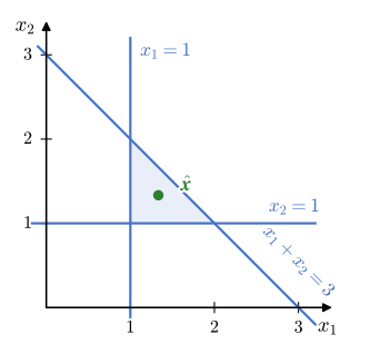
in the two unknowns \(x_1\) and \(x_2\) show both pictures at a small size. In the row picture, Figure 3.15.1, each equation is a line in the \(x_1x_2\) plane. Any two of the lines meet, at \((1, 1)\), \((2, 1)\) or \((1, 2)\), and the third line misses that point. No point lies on all three.
Figure 3.15.1: The row picture of Example 1: three lines that enclose a triangle and have no point in common, and the least-squares solution \(\hat{\bm x}\).
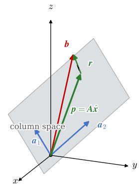
and in the column picture, Figure 3.15.2, it asks for the numbers \(x_1\) and \(x_2\) that make \(x_1\bm a_1 + x_2\bm a_2 = \bm b\). The columns \(\bm a_1 = (1, 0, 1)\) and \(\bm a_2 = (0, 1, 1)\) span a plane through the origin of space, the vectors whose third component is the sum of the first two. For \(\bm b = (1, 1, 3)\) the sum is \(2\), not \(3\), so \(\bm b\) lies above the plane.
Figure 3.15.2: The column picture of Example 1. As \(\bm x\) varies, \(\bm A\bm x\) runs over the plane of the columns \(\bm a_1\) and \(\bm a_2\), the column space, while \(\bm b\) lies outside it. The closest point \(\bm p = \bm A\hat{\bm x}\) is the foot of the perpendicular from the tip of \(\bm b\).
The normal equations
The column picture turns the minimum of 3.15.2 into geometry. The length \(\lvert\bm b - \bm A\bm x\rvert\) is the distance from the tip of \(\bm b\) to the point \(\bm A\bm x\) in the column space, and the shortest distance from a point to a plane is measured along the perpendicular, as for the point and the plane in Chapter 3.8. The best residual \(\hat{\bm r} = \bm b - \bm A\hat{\bm x}\) is therefore perpendicular to the column space, which means perpendicular to every column,
\[
\bm a_k\cdot\hat{\bm r} = \bm a_k^\mathsf{T}\hat{\bm r} = 0, \qquad k = 1, \dots, n
\]
The rows of \(\bm A^\mathsf{T}\) are the columns of \(\bm A\), so these \(n\) dot products are the \(n\) rows of the product \(\bm A^\mathsf{T}\hat{\bm r}\), and the conditions read \(\bm A^\mathsf{T}(\bm b - \bm A\hat{\bm x}) = \bm 0\). Multiplying out gives the normal equations
\[
\bm A^\mathsf{T}\bm A\,\hat{\bm x} = \bm A^\mathsf{T}\bm b
\tag{3.15.3}\]
named after the residual, which is normal to the column space. The matrix \(\bm A^\mathsf{T}\bm A\) is \(n\times n\) and symmetric, Chapter 3.10, so the \(m\) contradictory equations have become \(n\) equations in \(n\) unknowns, solved as in Chapter 3.12. When the columns of \(\bm A\) are linearly independent, Chapter 3.6, the solution is unique: \(\bm A^\mathsf{T}\bm A\bm x = \bm 0\) gives \(\bm x^\mathsf{T}\bm A^\mathsf{T}\bm A\bm x = \lvert\bm A\bm x\rvert^2 = 0\), so \(\bm A\bm x = \bm 0\) and \(\bm x = \bm 0\), and \(\bm A^\mathsf{T}\bm A\) is invertible, Chapter 3.11.
The perpendicular residual is also the shortest one. Any other \(\bm x\) leaves the residual \(\bm b - \bm A\bm x = \hat{\bm r} + \bm A(\hat{\bm x} - \bm x)\), whose second part lies in the column space and is perpendicular to the first. Multiplying out the dot product of the sum with itself, the mixed terms vanish and
with equality only for \(\bm A\bm x = \bm A\hat{\bm x}\). In the video, \(\bm x\) wanders and \(\bm A\bm x\) runs over the plane of the columns of Figure 3.15.2. The length of the residual falls and rises again, and it is least where the residual meets the plane at a right angle.
With a single column \(\bm a\) the column space shrinks to a line. Then \(\bm A^\mathsf{T}\bm A = \bm a\cdot\bm a\) and \(\bm A^\mathsf{T}\bm b = \bm a\cdot\bm b\) are numbers, and 3.15.3 gives
\[
\hat x = \frac{\bm a\cdot\bm b}{\bm a\cdot\bm a}
\tag{3.15.4}\]
the factor \(s\) of the projection in 3.6.7. Least squares is the projection of Chapter 3.6 with a plane, or a space of \(n\) columns, in place of the line, and \(\bm p = \bm A\hat{\bm x}\) is the projection of \(\bm b\) on the column space.
The derivative route of Chapter 3.8 arrives at the same equations. Multiplied out, the squared length of the residual is
\[
E(\bm x) = (\bm b - \bm A\bm x)^\mathsf{T}(\bm b - \bm A\bm x) = \bm b^\mathsf{T}\bm b - 2\,\bm x^\mathsf{T}\bm A^\mathsf{T}\bm b + \bm x^\mathsf{T}\bm A^\mathsf{T}\bm A\,\bm x
\]
where the two mixed terms are equal because a \(1\times 1\) matrix is its own transpose. \(E\) is quadratic in the unknowns, so its partial derivatives are linear in them, and setting the \(n\) derivatives to zero gives 3.15.3 again. Example 1 checks this with SymPy.
Write one equation per measurement, linear in the unknowns, and collect them as \(\bm A\bm x = \bm b\) with \(m > n\).
Form \(\bm A^\mathsf{T}\bm A\) and \(\bm A^\mathsf{T}\bm b\).
Solve the normal equations \(\bm A^\mathsf{T}\bm A\,\hat{\bm x} = \bm A^\mathsf{T}\bm b\).
Compute the residual \(\hat{\bm r} = \bm b - \bm A\hat{\bm x}\) and check that \(\bm A^\mathsf{T}\hat{\bm r} = \bm 0\).
Practise 3.15.4 below: the model \(y = c\,x\) has one column, the \(x\) of the points, and the least-squares slope is a projection.
Example 1: Three lines without a common point
Find the least-squares solution of the system of Figure 3.15.1,
whose solution is \(\hat x_1 = \hat x_2 = 4/3\). The residual follows from 3.15.1, \(\hat{\bm r} = \bm b - \bm A\hat{\bm x}\), and the check is \(\bm A^\mathsf{T}\hat{\bm r} = \bm 0\). As a second check, the derivative route sets \(\partial E/\partial x_1 = \partial E/\partial x_2 = 0\) with \(E = \lvert\bm b - \bm A\bm x\rvert^2\).
Code
x_1, x_2 = sp.symbols('x_1 x_2', real=True)AA = sp.Matrix([[1, 0], [0, 1], [1, 1]])bb = sp.Matrix([1, 1, 3])AtA = AA.T*AAAtb = AA.T*bbxx_hat = AtA.solve(Atb) # the n x n normal equations, n = 2rr = bb - AA*xx_hat # one miss per equationcheck = AA.T*rr # perpendicular to both columns# the derivative route: the same pointxx = sp.Matrix([x_1, x_2])E = (bb - AA*xx).dot(bb - AA*xx)sol = sp.solve([E.diff(x_1), E.diff(x_2)], [x_1, x_2])
The normal equations give the solution, the residual and the check
Each equation is missed by one third, and the least-squares point \((4/3, 4/3)\) is the centroid of the triangle in Figure 3.15.1. The residual \((-1, -1, 1)/3\) points along \(\bm a_1\times\bm a_2 = (-1, -1, 1)\), the normal of the column plane.
Practise the normal equations of a system with three equations and two unknowns below.
Example 2: The measured plate in matrix form
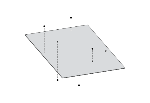
A probe measured the height \(z\) of a plate at six points, Figure 3.15.3, the data of Example 11 in Chapter 3.8, all in millimetres.
\(x\)
0
200
400
0
200
400
\(y\)
0
0
0
300
300
300
\(z\)
0.10
0.22
0.31
0.43
0.48
0.62
Fit the plane \(z = c_0 + c_1 x + c_2 y\) with the normal equations and compare with the derivative route of that chapter.
Figure 3.15.3: The least-squares plane of the plate and the six measured points, with heights and residuals drawn enlarged.
Each measured point gives one equation \(c_0 + c_1 x_i + c_2 y_i = z_i\), six equations in three unknowns,
The columns of \(\bm A\) are a column of ones, the \(x\) and the \(y\) of the points. The first row of \(\bm A^\mathsf{T}\hat{\bm r} = \bm 0\) is the dot product of the column of ones with the residual, \(\sum e_i = 0\), the property that Chapter 3.8 found from the derivative with respect to \(c_0\). The derivative route, 3.15.3 and the difference between the two are computed below.
Code
xs = [0, 200, 400, 0, 200, 400]ys = [0, 0, 0, 300, 300, 300]zs = [sp.Rational(h) for h in ('0.10', '0.22', '0.31', '0.43', '0.48', '0.62')]AA = sp.Matrix([[1, x_i, y_i] for x_i, y_i inzip(xs, ys)]) # one row per pointbb = sp.Matrix(zs)cc = (AA.T*AA).solve(AA.T*bb)ee = bb - AA*cc# the derivative route of the lines-and-planes chapterc_0, c_1, c_2 = sp.symbols('c_0 c_1 c_2', real=True)E =sum((z_i - (c_0 + c_1*x_i + c_2*y_i))**2for x_i, y_i, z_i inzip(xs, ys, zs))sol = sp.solve([E.diff(c) for c in (c_0, c_1, c_2)], [c_0, c_1, c_2])difference = cc - sp.Matrix([sol[c_0], sol[c_1], sol[c_2]])
The normal equations and the coefficients, with the difference from the derivative route, are
The two routes give the same exact fractions, \(z = 0.11 + 0.0005\,x + 0.001\,y\) to three digits: the plane of Example 11 and its flatness of 0.05 mm follow from either. The normal equations ask for no derivatives, and a seventh measured point would only add a row to \(\bm A\) and \(\bm b\).
NotePerpendicular residuals
The residuals here are vertical: only the height \(z\) is taken to carry errors, while \(x\) and \(y\) are exact. When every coordinate of the points is measured with error, the distance to minimise is the perpendicular distance to the plane, and the normal of the best plane is an eigenvector of a \(3\times 3\) matrix built from the points, Chapter 3.14.
Fitting curves
Nothing in Example 2 was special to planes. Least squares fits any model that is linear in its unknown coefficients,
with known functions \(f_k\), which may be as curved as we like. Each data point \((x_i, y_i)\) gives one row, and the matrix of the system, the design matrix, holds \(f_k(x_i)\) in row \(i\) and column \(k\),
For a polynomial the functions are \(1, x, \dots, x^{n-1}\), and for a signal that repeats with the angular frequency \(\omega\) they are \(1\), \(\cos\omega t\) and \(\sin\omega t\). Only the design matrix changes from model to model; 3.15.3 stays.
Example 3: A straight line through six points
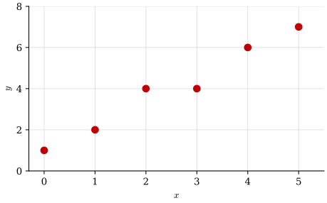
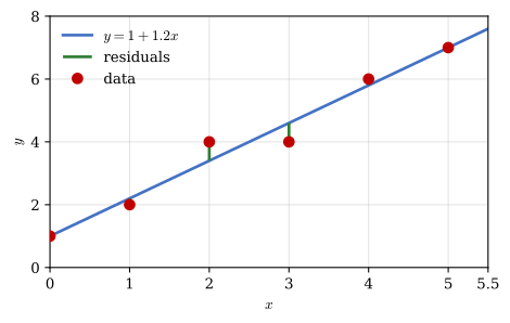
Fit the straight line \(y = c_0 + c_1 x\) to the six points of Figure 3.15.4, \(x_i = 0, 1, \dots, 5\) and \(y_i = 1, 2, 4, 4, 6, 7\).
Figure 3.15.4: Six points that lie near a straight line.
With \(f_1 = 1\) and \(f_2 = x\), the design matrix has a column of ones and the column of the \(x_i\). Its products are sums over the points,
The residuals add up to zero, as the column of ones demands, and the line passes exactly through the first and the last point. Figure 3.15.5 draws the fit over the data.
Code
x = np.array(xs, float)y = np.array(ys, float)c = np.array(cc, float).ravel()x_line = np.array([0, 5.5])fig, ax = plt.subplots(figsize=(5.0, 3.2))ax.plot(x_line, c[0] + c[1]*x_line, color='#4472c4', lw=2, label='$y = 1 + 1.2x$')# each residual as the vertical gap between a point and the lineax.vlines(x, c[0] + c[1]*x, y, color='#2e7d32', lw=2, label='residuals')ax.plot(x, y, 'o', color='#c00000', ms=7, zorder=5, label='data')ax.set_xlim(0, 5.5)ax.set_ylim(0, 8)ax.set_xticks([0, 1, 2, 3, 4, 5, 5.5], ['0', '1', '2', '3', '4', '5', '5.5'])ax.set_yticks([0, 2, 4, 6, 8])ax.set_xlabel('$x$')ax.set_ylabel('$y$')ax.grid(True, alpha=0.35)ax.legend(loc='upper left', frameon=False)fig.tight_layout()plt.show()
Figure 3.15.5: The least-squares line of Example 3 and the vertical residuals between the line and the points.
In the video the line moves over the points of Example 3. On every residual stands a square, so the shaded area is the sum that 3.15.2 makes least. The line passes a point where the sum is smaller than at the start and still not least, and it settles at \(c_0 = 1\), \(c_1 = 1.2\), where no move of the line shrinks the total area further.
Practise the straight-line fit below. Four points give a \(4\times 2\) design matrix, and the normal equations are built from the four sums \(m\), \(\sum x_i\), \(\sum x_i^2\) and \(\sum x_i y_i\) together with \(\sum y_i\).
Example 4: A parabola through six points
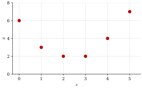
Fit the parabola \(y = c_0 + c_1 x + c_2 x^2\) to the six points of Figure 3.15.6, \(x_i = 0, 1, \dots, 5\) and \(y_i = 6, 3, 2, 2, 4, 7\).
Figure 3.15.6: Six points that lie near a parabola.
The design matrix gains the column of the \(x_i^2\), and the normal equations hold sums of powers up to \(x^4\),
The parabola \(y \approx 5.93 - 3.52x + 0.75x^2\) misses no point by more than 0.16. Every column we add enlarges the column space, so the least sum of squares can only fall. In the video the points of Example 4 are fitted with one to six columns, the polynomials of degree 0 to 5. The sum drops sharply at the third column, where the model first has the shape of the data, and barely after it. With six columns \(\bm A\) is square and invertible, the curve passes through every point and the sum is zero, but the curve now follows the scatter of the points as well as their trend and bends between them. A good model has few columns compared with the number of points.
Practise the design matrix below: write \(\bm A\) for a model and a set of points, row by row, as a list such as [[1, 0, 0], [1, 1, 1], [1, 2, 4]].
Example 5: A daily temperature cycle
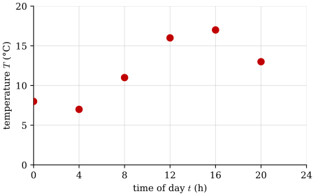
A thermometer outdoors reads the temperatures of Figure 3.15.7 every four hours,
\(t\) (h)
0
4
8
12
16
20
\(T\) (°C)
8
7
11
16
17
13
Fit the daily cycle \(T(t) = c_0 + c_1\cos\omega t + c_2\sin\omega t\) with \(\omega = 2\pi/24\ \text{h}^{-1}\), and find the mean temperature, the amplitude of the cycle and the time of day of the maximum.
Figure 3.15.7: Six temperatures read over one day.
The design matrix has the rows \((1, \cos\omega t_i, \sin\omega t_i)\). At the six times, \(\omega t_i\) runs through \(0°, 60°, \dots, 300°\), so
The columns are orthogonal, as they are for any samples evenly spread over one period, so \(\bm A^\mathsf{T}\bm A\) is diagonal and each normal equation holds one unknown,
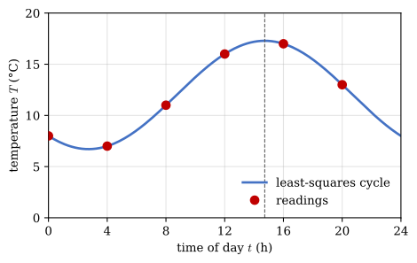
The day averages 12 °C and swings 5.3 °C to either side, with the warmest moment at 14.7 h, about a quarter to three in the afternoon. The model \(T_0 + R\cos(\omega(t - t_{\max}))\) is not linear in \(t_{\max}\); written with a cosine and a sine it is linear in \(c_1\) and \(c_2\), and least squares applies. A model such as \(y = a\,e^{kx}\) is made linear the same way, by fitting \(\ln y = \ln a + kx\). Figure 3.15.8 draws the cycle through the readings.
Figure 3.15.8: The fitted daily cycle of Example 5 and the six readings. The dashed line marks the maximum at \(t_{\max} \approx 14.7\) h.
Example 6: The point nearest to several lines
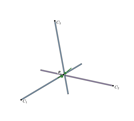
Example 6 of Chapter 3.8 found the point \(\bm p\) nearest to three sight lines, Figure 3.15.9, by setting derivatives to zero. The cameras are at \(C_1 = (6, 0, 0)\), \(C_2 = (0, 6, 0)\) and \(C_3 = (0, 0, 5)\) and look along \(\bm v_1 = (-4, 2, 1)\), \(\bm v_2 = (2, -4, 1)\) and \(\bm v_3 = (2, 2, -3)\). Write the problem on the form \(\bm A\bm p = \bm b\), solve it with the normal equations, and add a fourth camera at \(C_4 = (6, 6, 0)\) looking along \(\bm v_4 = (-3, -3, 1)\).
Figure 3.15.9: The three sight lines of Example 6 in Chapter 3.8 and the least-squares point \(\bm p\), with the distance vectors drawn enlarged.
The distance vector from line \(i\) to \(\bm p\) is what is left of \(\bm a = \bm p - \bm r_{C_i}\) after its projection on the unit vector \(\bm e_i = \bm v_i/\lvert\bm v_i\rvert\) is removed, \(\bm d_i = \bm a - (\bm a\cdot\bm e_i)\,\bm e_i\). The projection is a matrix product: \(\bm e_i\bm e_i^\mathsf{T}\) is a \(3\times 1\) column times a \(1\times 3\) row, a \(3\times 3\) matrix, and \((\bm e_i\bm e_i^\mathsf{T})\bm a = \bm e_i(\bm e_i^\mathsf{T}\bm a) = (\bm a\cdot\bm e_i)\,\bm e_i\) is the cheap projection of 3.6.8. With
\[
\bm P_i = \bm I - \bm e_i\bm e_i^\mathsf{T}
\]
the distance vector is \(\bm d_i = \bm P_i(\bm p - \bm r_{C_i})\). A point on every line would have \(\bm d_i = \bm 0\) for all \(i\), three equations \(\bm P_i\bm p = \bm P_i\bm r_{C_i}\) per line, and stacked they form an overdetermined system with nine rows,
Its residual is the stack of the three distance vectors, so \(\lvert\bm r\rvert^2 = \sum\lvert\bm d_i\rvert^2\) is the sum that Chapter 3.8 minimised. The fourth camera adds three rows. \(\bm A^\mathsf{T}\bm A\) and \(\bm A^\mathsf{T}\bm b\) come out as sums over the lines, since \(\bm P_i\) is symmetric and \(\bm P_i\bm P_i = \bm P_i\) (removing the part along \(\bm e_i\) twice removes nothing more), so the normal equations read
cameras = [sp.Matrix([6, 0, 0]), sp.Matrix([0, 6, 0]), sp.Matrix([0, 0, 5]), sp.Matrix([6, 6, 0])]sight = [sp.Matrix([-4, 2, 1]), sp.Matrix([2, -4, 1]), sp.Matrix([2, 2, -3]), sp.Matrix([-3, -3, 1])]def stacked(n):"""A and b of the first n lines: the block P_i removes the part along line i.""" PP = [sp.eye(3) - vv*vv.T/vv.dot(vv) for vv in sight[:n]] # e e^T = v v^T / v.v AA = sp.Matrix.vstack(*PP) bb = sp.Matrix.vstack(*[P*rr_C for P, rr_C inzip(PP, cameras[:n])])return AA, bbAA, bb = stacked(3)pp_3 = (AA.T*AA).solve(AA.T*bb)same_as_sums = AA.T*AA -sum((sp.eye(3) - vv*vv.T/vv.dot(vv) for vv in sight[:3]), sp.zeros(3))AA, bb = stacked(4)pp_4 = (AA.T*AA).solve(AA.T*bb)dd_4 = [(bb - AA*pp_4)[3*i:3*i +3, 0].norm() for i inrange(4)]
With the three lines of Chapter 3.8, and with the fourth line added, the normal equations give
The three-line point is the exact point \((244/115, 244/115, 53/46)\) of Chapter 3.8. The fourth sight line passes close to it, within 0.10, and moves the point by less than 0.05. In matrix form a further measurement is three more rows and one more term in each sum, and the system stays \(3\times 3\) however many lines are measured.
Solving least-squares problems in practice
The normal equations are the way to solve by hand and to reason about least squares, and they serve for small, well-scaled problems. On a computer, forming \(\bm A^\mathsf{T}\bm A\) squares the condition number of the problem, Chapter 3.12: \(\kappa(\bm A^\mathsf{T}\bm A) = \kappa(\bm A)^2\).
Code
x = np.arange(6.0)y = np.array([6, 3, 2, 2, 4, 7.0])conds = []for n in (2, 3, 5): A = np.vander(x, n, increasing=True) # columns 1, x, ..., x^(n-1) conds.append([n, np.linalg.cond(A), np.linalg.cond(A.T @ A)])conds = np.array(conds)A = np.vander(x, 3, increasing=True)c, res, rank, sv = np.linalg.lstsq(A, y, rcond=None)
For the points of Example 4 fitted with \(n\) columns, the condition numbers are
With five columns \(\bm A^\mathsf{T}\bm A\) loses about seven of the sixteen digits of a double-precision number before the solution starts. np.linalg.lstsq(A, b, rcond=None) avoids \(\bm A^\mathsf{T}\bm A\) altogether: it factorises \(\bm A\) itself into orthogonal and triangular factors and solves 3.15.2 with the condition number of \(\bm A\). It returns the coefficients, the least sum of squares, the rank of \(\bm A\) and its singular values, and for the parabola of Example 4 it gives
the coefficients and the sum \(3/35 \approx 0.0857\) of Example 4. In SymPy, exact arithmetic has no round-off and (AA.T*AA).solve(AA.T*bb) is safe, as in the examples above.