“I recommend this method to you for imitation. You will hardly ever again eliminate directly, at least not when you have more than 2 unknowns. The indirect procedure can be done while half asleep, or while thinking about other things.”
— Carl Friedrich Gauss, letter to Christian Ludwig Gerling, 26 December 1823, translated by George E. Forsythe (1951)
Several linear equations that hold at the same time form a linear system. With the coefficients collected in a matrix \(\bm A\), the unknowns in a vector \(\bm x\) and the right-hand sides in a vector \(\bm b\), every linear system takes one form,
\[
\boxed{\bm A\bm x = \bm b}
\tag{3.12.1}\]
The product \(\bm A\bm x\) is the map of Chapter 3.10 applied to \(\bm x\), so to solve the system is to find the vector that \(\bm A\) sends to \(\bm b\). The direct elimination that Gauss advises against in the letter is how computers solve most systems today, and his indirect method lives on in the iterative solvers for the very largest ones.
Linear equations
An equation in the unknowns \(x\) and \(y\) is linear when each unknown is only multiplied by a number and the terms are added, as in
\[
6x + 2y = 10
\]
Powers, roots, products of unknowns and functions of them are not allowed, so \(6x^2 + 2y = 10\), \(x + 2\sqrt y = 1\) and \(xy + y = 3\) are not linear. The pair \(x = 1\), \(y = 2\) satisfies the equation and is a solution. So is \(x = 0\), \(y = 5\), and so is every point of the line \(y = 5 - 3x\): one equation in two unknowns leaves one unknown free.
A linear system of \(m\) equations in \(n\) unknowns \(x_1, \dots, x_n\) has the coefficients \(a_{ij}\), where \(i\) numbers the equation and \(j\) the unknown, and the right-hand sides \(b_i\),
The \(m\times n\) matrix \(\bm A\) is the coefficient matrix, \(\bm b\) the right-hand side and \(\bm x\) the solution vector. Row \(i\) of \(\bm A\) times \(\bm x\), by the row-times-column rule of Chapter 3.10, is the left-hand side of equation \(i\), and column \(j\) of \(\bm A\) holds the coefficients of the unknown \(x_j\). A system with \(\bm b = \bm 0\) is homogeneous.
The system is square when \(m = n\), overdetermined when there are more equations than unknowns, \(m > n\), and underdetermined when there are fewer, \(m < n\). Square systems are by far the most common, and a linear system without a qualifier is a square one. The overdetermined system returns in Chapter 3.15.
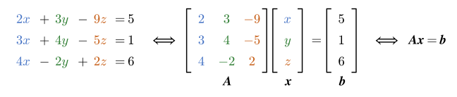
The coefficients of \(x\) form the first column of \(\bm A\), those of \(y\) the second and those of \(z\) the third, Figure 3.12.1,
\[
\bm A = \begin{bmatrix} 2 & 3 & -9 \\ 3 & 4 & -5 \\ 4 & -2 & 2 \end{bmatrix}, \qquad
\bm x = \begin{bmatrix} x \\ y \\ z \end{bmatrix}, \qquad
\bm b = \begin{bmatrix} 5 \\ 1 \\ 6 \end{bmatrix}
\]
and as a check, \(\bm A\bm x - \bm b\) must give back the three equations with everything moved to the left.
Figure 3.12.1: The system of Example 1 on matrix form. Each unknown keeps its colour: column \(j\) of \(\bm A\) holds the coefficients of the \(j\)th unknown, and row \(i\) is equation \(i\).
SymPy reads the matrices off the equations with sp.linear_eq_to_matrix.
Code
x, y, z = sp.symbols('x y z', real=True)eqs = [sp.Eq(2*x +3*y -9*z, 5), sp.Eq(3*x +4*y -5*z, 1), sp.Eq(4*x -2*y +2*z, 6)]# the order of the unknowns in the list fixes the order of the columnsAA, bb = sp.linear_eq_to_matrix(eqs, [x, y, z])xx = sp.Matrix([x, y, z])residual = AA*xx - bb
The matrices and the check are
\[ \begin{aligned}\bm A &= \left[\begin{matrix}2 & 3 & -9\\3 & 4 & -5\\4 & -2 & 2\end{matrix}\right],\quad \bm b = \left[\begin{matrix}5\\1\\6\end{matrix}\right]\\ \bm A\bm x - \bm b &= \left[\begin{matrix}2 x + 3 y - 9 z - 5\\3 x + 4 y - 5 z - 1\\4 x - 2 y + 2 z - 6\end{matrix}\right]\end{aligned} \]
Each row of \(\bm A\bm x - \bm b\) is one of the equations written as “left-hand side minus right-hand side equals zero”.
The row picture
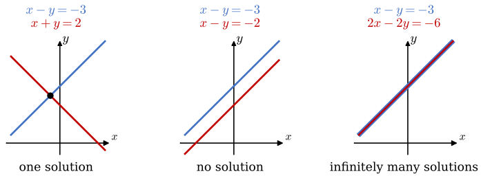
Each equation in two unknowns is a line in the plane, and a solution of the system is a point on every line at once. Two lines either cross, run parallel or coincide, so a system of two equations has exactly one solution, none, or infinitely many, Figure 3.12.2.
Figure 3.12.2: The row picture: each equation is a line. The lines cross in one point (left), are parallel with no common point (middle), or are the same line (right).
The left-hand sides decide whether the lines cross. In the middle and on the right of Figure 3.12.2 the second row of \(\bm A\) is a multiple of the first, the lines have the same direction, and \(\det\bm A = 0\). The right-hand sides then decide between parallel lines and one line. When \(\det\bm A \ne 0\) the map can be undone, Chapter 3.11, and the system has one solution \(\bm x = \bm A^{-1}\bm b\) for every \(\bm b\).
In three unknowns each equation is a plane. Three planes have one point in common, a whole line, a whole plane, or no point at all.
The column picture
Read by columns, as in Chapter 3.10, the product \(\bm A\bm x\) is a combination of the columns \(\bm a_1, \dots, \bm a_n\) of \(\bm A\) with the unknowns as weights,
The system asks for the weights that combine the columns into \(\bm b\). As a map, \(\bm A\) sends \(\bm i\) to \(\bm a_1\) and \(\bm j\) to \(\bm a_2\), and the solution is the vector \(\bm x\) that lands on \(\bm b\). In the video the plane is carried by \(\bm A\) of the left system in Figure 3.12.2, and \(\bm x\) arrives at \(\bm b\), which stays where it is. The same arrival reads as \(x_1\bm a_1\) followed by \(x_2\bm a_2\).
All combinations of the columns together form the column space of \(\bm A\), everything the map can reach. The number of linearly independent columns, Chapter 3.6, is the rank of \(\bm A\), and it counts the directions the column space spans: a line for rank 1, a plane for rank 2.
\(\bm A\bm x = \bm b\) has a solution exactly when \(\bm b\) lies in the column space of \(\bm A\).
The vectors that \(\bm A\) sends to \(\bm 0\) form the null space of \(\bm A\). It always holds \(\bm x = \bm 0\). When it also holds a vector \(\bm n \ne \bm 0\), then \(n_1\bm a_1 + \dots + n_n\bm a_n = \bm 0\) is a dependence between the columns, and a solution is no longer unique. If \(\bm x_p\) solves the system, so does \(\bm x_p + t\bm n\) for every number \(t\), since \(\bm A(\bm x_p + t\bm n) = \bm b + t\,\bm 0\). All solutions are then
\[
\bm x = \bm x_p + t\bm n, \qquad \bm A\bm x_p = \bm b, \qquad \bm A\bm n = \bm 0
\tag{3.12.3}\]
with one free number \(t\) for each independent vector of the null space.
The singular map in the video flattens the plane onto the line of its columns, and its determinant falls to zero. The vector \(\bm n\) lands on the origin. The vector \(\bm b\) lies off the line, and no vector of the plane is sent there.
For a square matrix both questions have one answer. When \(\det\bm A \ne 0\) the columns span everything, every \(\bm b\) is reached, and only \(\bm 0\) is sent to \(\bm 0\). When \(\det\bm A = 0\) the column space is smaller, and the null space holds more than \(\bm 0\). The homogeneous system \(\bm A\bm x = \bm 0\) always has the solution \(\bm x = \bm 0\), and it has others exactly when \(\det\bm A = 0\).
The second half of Grant Sanderson’s episode in Chapter 3.11 draws the column space and the null space in this way, as what a map reaches and what it flattens onto the origin, in the plane and in space.
Example 2: Columns that combine to b
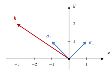
Figure 3.12.3: The columns \(\bm a_1 = (1, 1)^\mathsf{T}\) and \(\bm a_2 = (-1, 1)^\mathsf{T}\) and the right-hand side \(\bm b = (-3, 2)^\mathsf{T}\).
The system \(x_1 - x_2 = -3\), \(x_1 + x_2 = 2\) is the one on the left in Figure 3.12.2. Find the weights that combine its columns into \(\bm b\), Figure 3.12.3.
The sum of the two rows gives \(2x_1 = -1\) and their difference \(2x_2 = 5\), so \(x_1 = -\tfrac12\) and \(x_2 = \tfrac52\). The check is that \(x_1\bm a_1 + x_2\bm a_2 - \bm b = \bm 0\).
Code
AA = sp.Matrix([[1, -1], [1, 1]])bb = sp.Matrix([-3, 2])x1, x2 = sp.symbols('x1 x2', real=True)# the unknowns are the weights of the two columnssol = sp.solve(AA*sp.Matrix([x1, x2]) - bb, [x1, x2])check = sol[x1]*AA[:, 0] + sol[x2]*AA[:, 1] - bb
Half of \(\bm a_1\) backwards and two and a half of \(\bm a_2\) reach \(\bm b\), the path the first video draws in green.
Practise the column picture below. Once the weights are right, \(x_1\bm a_1\) and \(x_2\bm a_2\) are drawn tip to tail.
Example 3: Dependent columns
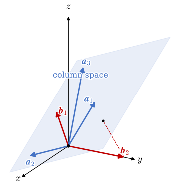
Figure 3.12.4: The columns \(\bm a_1\), \(\bm a_2\) and \(\bm a_3\) lie in one plane, the column space. The right-hand side \(\bm b_1\) lies in it, and \(\bm b_2\) does not.
The vectors \(\bm a_1 = (1, 2, 3)^\mathsf{T}\), \(\bm a_2 = (2, -1, 0)^\mathsf{T}\) and \(\bm a_3 = (4, 3, 6)^\mathsf{T}\) of the linear dependence in Chapter 3.6 are the columns of \(\bm A\), Figure 3.12.4. Solve \(\bm A\bm x = \bm b_1\) with \(\bm b_1 = (3, 1, 3)^\mathsf{T}\) and \(\bm A\bm x = \bm b_2\) with \(\bm b_2 = (0, 3, 0)^\mathsf{T}\).
The dependence \(\bm a_3 = 2\bm a_1 + \bm a_2\) found there gives \(2\bm a_1 + \bm a_2 - \bm a_3 = \bm 0\), so the null space holds \(\bm n = (2, 1, -1)^\mathsf{T}\), and the rank is 2. The right-hand side \(\bm b_1 = \bm a_1 + \bm a_2\) is reached with the weights \(\bm x_p = (1, 1, 0)^\mathsf{T}\), and by 3.12.3 all solutions are
\[
\bm x = \begin{bmatrix}1\\1\\0\end{bmatrix} + t\begin{bmatrix}2\\1\\-1\end{bmatrix}
\]
The column space is the plane through the origin with the normal \(\bm a_1\times\bm a_2 = (3, 6, -5)^\mathsf{T}\), Chapter 3.7. A right-hand side lies in it when it is perpendicular to the normal. For \(\bm b_1\) the dot product is \(9 + 6 - 15 = 0\), for \(\bm b_2\) it is \(18\), so \(\bm A\bm x = \bm b_2\) has no solution.
In SymPy, rank and nullspace answer the questions about \(\bm A\), and sp.linsolve returns every solution of a system, as a set that is empty when there is none.
The rank, the null space and the two solution sets are
\[ \begin{aligned}\operatorname{rank}\bm A &= 2,\quad \bm n = \left[\begin{matrix}-2\\-1\\1\end{matrix}\right]\\ \bm A\bm x = \bm b_1 &: \ \left[\begin{matrix}1 - 2 x_{3}\\1 - x_{3}\\x_{3}\end{matrix}\right]\\ \bm A\bm x = \bm b_2 &: \ \emptyset\end{aligned} \]
SymPy keeps \(x_3\) as the free number. With \(x_3 = -t\) its solution is \((1 + 2t,\ 1 + t,\ -t)^\mathsf{T}\), the line found by hand, and its null vector is \(-\bm n\), the same direction.
Practise a singular system in the plane below. The two columns are parallel, so the null vector and one particular solution give all solutions.
Ill-conditioning
When \(\det\bm A\) is close to zero, the lines of the row picture are close to parallel. A small change of \(\bm A\) or \(\bm b\) then moves their crossing far, and the system is called ill-conditioned. In the video both systems get the same small change \(\varepsilon\) in one right-hand side. The steep crossing on the left hardly moves; the crossing of the nearly parallel lines on the right moves about thirty times as far as \(\varepsilon\).
The condition number \(\kappa(\bm A)\) measures this. A relative change of \(\bm b\) can grow into a relative change of \(\bm x\) up to \(\kappa(\bm A)\) times larger. For the steep pair of the video the condition number is 1, for the nearly parallel pair about 82, and NumPy computes it with np.linalg.cond(A). A small determinant alone is no measure: \(0.1\,\bm A\) has a determinant a hundred times smaller in the plane and the same condition number. An ill-conditioned system usually points back at the model, at two equations that say almost the same thing.
Example 4: Two almost equal systems
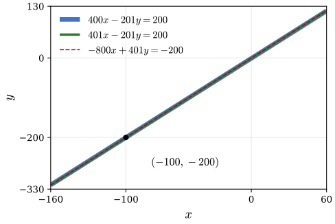
Figure 3.12.5: The lines of the two systems near the solution \((-100, -200)\) of the first one. At this scale all three lines lie on top of each other.
A change in the third digit of one coefficient moves the solution four hundred times further from the origin. The second matrix is almost singular: its determinant passes zero at \(a_{11} \approx 400.998\), just below 401, where the two lines are parallel and the solution has run off to infinity and back.
Modelling with linear systems
The work in a model lies in writing the equations. Once they stand on the page, sp.solve takes them as they are written, with no need to collect \(\bm A\) and \(\bm b\) by hand first. How a solver reaches the answer is the subject of the next section.
Example 5: A jar of cream
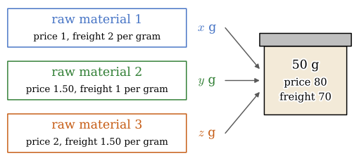
Figure 3.12.6: Three raw materials with their prices and freight per gram, mixed into a jar of 50 g that costs 80 in raw materials and 70 in freight.
A jar of skin cream weighs 50 g and is made of three raw materials, Figure 3.12.6. They cost 1, 1.50 and 2 kronor per gram, and their freight costs 2, 1 and 1.50 kronor per gram. The raw materials of one jar cost 80 kronor and their freight 70 kronor. How many grams of each raw material does a jar hold?
With \(x\), \(y\) and \(z\) grams of the three raw materials, the weight, the price and the freight give one equation each,
\[
\begin{aligned}
x + y + z &= 50 \\
x + 1.5y + 2z &= 80 \\
2x + y + 1.5z &= 70
\end{aligned}
\]
In SymPy the decimals are written as fractions, so that the answer is exact.
Code
x, y, z = sp.symbols('x y z', real=True)half = sp.Rational(1, 2)sol = sp.solve([sp.Eq(x + y + z, 50), sp.Eq(x + (1+ half)*y +2*z, 80), sp.Eq(2*x + y + (1+ half)*z, 70)], [x, y, z])
The amounts in grams are
\[ x = 10,\quad y = 20,\quad z = 20 \]
They add up to 50 g, and \(10 + 1.5\cdot 20 + 2\cdot 20 = 80\) kronor as the jar’s price requires.
Example 6: Three liquids
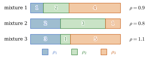
Figure 3.12.7: Three mixtures of the same three liquids in the volume ratios 1:2:4, 2:3:1 and 3:1:5, with the densities of the mixtures.
Three liquids mixed in the volume ratio 1:2:4 give a mixture of density 0.9. Mixed 2:3:1 they give 0.8, and mixed 3:1:5 they give 1.1, Figure 3.12.7. Find the densities \(\rho_1\), \(\rho_2\) and \(\rho_3\) of the three liquids.
The density of a mixture is its mass over its volume. One part of volume of liquid \(k\) has the mass \(\rho_k\), so the first mixture, seven parts in all, gives \((\rho_1 + 2\rho_2 + 4\rho_3)/7 = 0.9\). With the volumes multiplied out, the three mixtures give
r1, r2, r3 = sp.symbols('rho1 rho2 rho3', positive=True)# each mixture: the masses of its parts add up to its volume times its densitysol = sp.solve([sp.Eq(1*r1 +2*r2 +4*r3, 7*sp.Rational(9, 10)), sp.Eq(2*r1 +3*r2 +1*r3, 6*sp.Rational(8, 10)), sp.Eq(3*r1 +1*r2 +5*r3, 9*sp.Rational(11, 10))], [r1, r2, r3])
The second liquid is the light one, which is why the mixture with the most of it, 2:3:1, has the lowest density.
Example 7: Temperatures in a plate
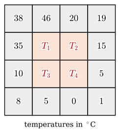
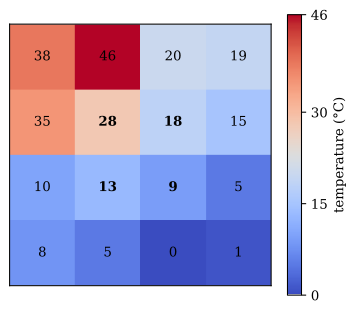
Figure 3.12.8: A square plate divided into sixteen squares. The temperatures of the twelve squares along the edge are known, the four inner ones are not.
A square plate is divided into four rows of four squares, Figure 3.12.8. The temperatures of the squares along the edge are known. Find the temperatures \(T_1\) to \(T_4\) of the four inner squares, assuming that the temperature of an inner square is the mean of the temperatures of its four neighbours, above, below, left and right.
Figure 3.12.9 draws the whole plate with the computed temperatures filled in. Warm from the upper left, cold toward the lower right, each inner value lies between its neighbours.
Code
grid = np.array([[38, 46, 20, 19], [35, sol[T1], sol[T2], 15], [10, sol[T3], sol[T4], 5], [8, 5, 0, 1]], dtype=float)fig, ax = plt.subplots(figsize=(4.4, 3.8))im = ax.imshow(grid, cmap='coolwarm', vmin=0, vmax=46)for i inrange(4):for j inrange(4):# the four computed values in bold, the given ones plain bold =1<= i <=2and1<= j <=2 ax.text(j, i, f'{grid[i, j]:.0f}', ha='center', va='center', fontweight='bold'if bold else'normal')ax.set_xticks([])ax.set_yticks([])cb = fig.colorbar(im, ax=ax, ticks=[0, 15, 30, 46])cb.set_label('temperature (°C)')plt.show()
Figure 3.12.9: The plate of Example 7 with the computed inner temperatures in bold.
The rule that a value is the mean of its neighbours is the finite difference form of the equation of steady heat conduction. With a finer grid there are more unknowns and the same kind of system; Chapter 13.7 solves the same problem with finite elements.
Solving a linear system
With the inverse
When \(\det\bm A \ne 0\), multiplying \(\bm A\bm x = \bm b\) from the left by \(\bm A^{-1}\) of Chapter 3.11 gives \(\bm x = \bm A^{-1}\bm b\). For Example 2 the \(2\times 2\) formula gives
which is the quickest route for a \(2\times 2\) system by hand. For larger systems the inverse takes about three times the work of solving the system once, collects more round-off, and is rarely wanted for its own sake. A computer eliminates instead.
Gauss elimination
Three operations on the equations of a system leave its solutions unchanged: swapping two equations, multiplying an equation by a number other than zero, and adding a multiple of one equation to another. They are the elementary row operations. Take
which gives \(y = -\tfrac25\), and with it in the first equation, \(2x - \tfrac{12}{5} = 3\) and \(x = \tfrac{27}{10}\).
Every combination of the two equations is satisfied by the solution, so in the row picture it is a line through the crossing point. In the video the row operation turns the second line about the crossing until \(x\) has dropped out and the line lies horizontal, \(y = -\tfrac25\).
The work is done on the augmented matrix \([\bm A \mid \bm b]\), the coefficient matrix with \(\bm b\) as an extra column, since only the numbers change. The elimination goes through the columns from left to right. In column \(j\), the number \(a_{jj}\) on the diagonal is the pivot, and row \(i\) below it loses the multiple
\[
l_{ij} = \frac{a_{ij}}{a_{jj}}
\tag{3.12.4}\]
of row \(j\), which makes its entry in column \(j\) zero. When all columns are done, every entry below the diagonal is zero and the matrix is upper triangular, in row echelon form. The last equation then holds one unknown, the one above it two, and back substitution solves them from the bottom up.
Adding a multiple of one row to another does not change the determinant, Chapter 3.11, and the determinant of a triangular matrix is the product of its diagonal. The determinant therefore comes for free: \(\det\bm A\) is the product of the pivots.
A pivot of zero stops the elimination, and a pivot close to zero divides by a small number and magnifies round-off. Before each column, partial pivoting swaps the row with the largest entry of the column, in absolute value, into the pivot place. Every library solver does this.
Write the augmented matrix \([\bm A \mid \bm b]\).
For each column \(j\) from the left, subtract \(l_{ij} = a_{ij}/a_{jj}\) times row \(j\) from every row \(i\) below it.
Solve the last equation for the last unknown, and work upward, inserting the unknowns already found.
Check that \(\bm A\bm x = \bm b\).
Elimination on \(n\) equations takes about \(\tfrac23 n^3\) multiplications and additions, so a system ten times larger takes a thousand times longer. Large systems come from models built of many small parts, such as the trusses of Chapter 8.15 and the finite elements of Chapter 13.2, where \(n\) reaches millions and only a computer eliminates.
by Gauss elimination, and find \(\det\bm A\). In the video each equation is a plane through the solution, and each row operation turns one plane about that point.
In column 1 the pivot is 2, and the multipliers are \(\tfrac42 = 2\) and \(\tfrac62 = 3\). In column 2 the pivot is \(-2\), and the multiplier is \(\tfrac{-4}{-2} = 2\),
SymPy’s own determinant and the residual confirm the result,
\[ \det\bm A = 28,\qquad \bm A\bm x - \bm b = \left[\begin{matrix}0\\0\\0\end{matrix}\right] \]
and the last column of the eliminated matrix, \((2, -1, 2)^\mathsf{T}\), is \(\bm b\) after the same row operations.
Practise Gauss elimination below. The problems are made so that every multiplier is a whole number.
LU factorisation
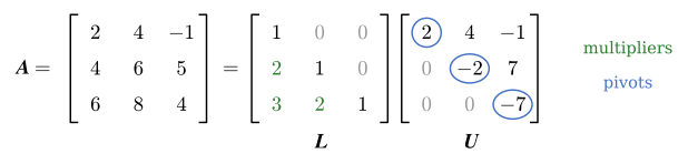
The multipliers of the elimination need not be thrown away. Collected below the diagonal of a matrix with ones on its diagonal, they form the lower triangular matrix \(\bm L\). The eliminated matrix is the upper triangular \(\bm U\), and together
\[
\bm A = \bm L\bm U
\tag{3.12.5}\]
With the factors in hand, \(\bm A\bm x = \bm L(\bm U\bm x) = \bm b\) splits into two triangular systems,
\[
\bm L\bm y = \bm b, \qquad \bm U\bm x = \bm y
\tag{3.12.6}\]
The first is solved from the top down by forward substitution, which repeats on \(\bm b\) the row operations of the elimination, and the second from the bottom up by back substitution. The factorisation takes the \(\tfrac23 n^3\) operations of the elimination; each pair of substitutions takes about \(2n^2\). A model that is solved for many right-hand sides with the same \(\bm A\) is factored once, and every further \(\bm b\) costs only the substitutions. With partial pivoting the rows are swapped on the way, and the factorisation is \(\bm P\bm A = \bm L\bm U\) with a permutation matrix \(\bm P\) that records the swaps.
Example 9: One factorisation, two right-hand sides
Figure 3.12.10: The LU factorisation of \(\bm A\) of Example 8. The multipliers of the elimination stand below the diagonal of \(\bm L\), and the pivots on the diagonal of \(\bm U\).
Factor \(\bm A\) of Example 8 as \(\bm L\bm U\), Figure 3.12.10, and use the factors to solve \(\bm A\bm x = \bm b\) both for \(\bm b_1 = (2, 3, 6)^\mathsf{T}\) and for \(\bm b_2 = (5, 15, 18)^\mathsf{T}\).
The multipliers of Example 8 were \(l_{21} = 2\), \(l_{31} = 3\) and \(l_{32} = 2\), and \(\bm U\) is the eliminated matrix,
For \(\bm b_1\) the substitutions repeat Example 8. For \(\bm b_2\), forward substitution in \(\bm L\bm y = \bm b_2\) gives \(y_1 = 5\), \(y_2 = 15 - 2\cdot 5 = 5\) and \(y_3 = 18 - 3\cdot 5 - 2\cdot 5 = -7\), and back substitution in \(\bm U\bm x = \bm y\) gives
With numbers, scipy.linalg.lu_factor factors once and scipy.linalg.lu_solve substitutes for as many right-hand sides as we give it, here the two as the columns of one array.
Code
A = np.array(AA, dtype=float)B = np.array(bb1.row_join(bb2), dtype=float) # one right-hand side per columnlu, piv = scipy.linalg.lu_factor(A) # pivoting: row 3 with its 6 goes firstX = scipy.linalg.lu_solve((lu, piv), B)
where \(\bm A_k\) is \(\bm A\) with column \(k\) replaced by \(\bm b\). For the first system of Example 4, \(x = \det\begin{bmatrix}200 & -201\\-200 & 401\end{bmatrix}/(-400) = (80\,200 - 40\,200)/(-400) = -100\). The rule is handy for a \(2\times 2\) system by hand and in proofs. It needs \(n + 1\) determinants, and beyond three unknowns elimination is far cheaper. Grant Sanderson shows why the rule holds: \(\det\bm A_k\) is the area of a parallelogram after the map, and the area before the map is \(x_k\).
An iterative method
Elimination reaches the answer after a fixed number of operations, but it needs all of \(\bm A\) in memory and changes it as it goes. In the very largest systems most entries of \(\bm A\) are zero, and elimination fills them in. An iterative method starts from a guess \(\bm x_0\) and improves it step by step, and it uses \(\bm A\) only to multiply vectors. The quality of a guess is measured by its residual
\[
\bm r = \bm b - \bm A\bm x
\]
which is zero at the solution. We stop when \(|\bm r|\) is small enough, which also lets us stop at the accuracy the model deserves.
Steepest descent is the simplest of these methods. Let \(\bm A\) be symmetric, with \(\bm x^\mathsf{T}\bm A\bm x > 0\) for every \(\bm x \ne \bm 0\). Then the solution of \(\bm A\bm x = \bm b\) is the lowest point of the bowl
\[
f(\bm x) = \tfrac12\,\bm x^\mathsf{T}\bm A\bm x - \bm b^\mathsf{T}\bm x
\]
since setting its partial derivatives to zero, as for the least-squares problem of Chapter 3.8, gives \(\bm A\bm x - \bm b = \bm 0\). The vector of these partial derivatives is \(-\bm r\), so the residual points the steepest way down. From \(\bm x_i\) we walk along \(\bm r_i\) as far as \(f\) decreases. Multiplied out with the symmetry of \(\bm A\),
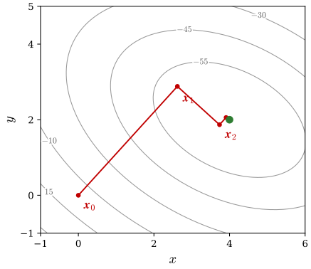
Each step turns at a right angle to the last, so the path zigzags down the bowl. The conjugate gradient method, a refinement that chooses better directions, is a common iterative solver for large finite element models.
Example 10: Steepest descent
Figure 3.12.11: The level curves of \(f(\bm x)\) for Example 10, the steps of steepest descent from \(\bm x_0 = \bm 0\) in red and the solution in green.
by steepest descent from \(\bm x_0 = \bm 0\), Figure 3.12.11, until \(\bm r^\mathsf{T}\bm r < 10^{-12}\).
The matrix is symmetric, and \(\bm x^\mathsf{T}\bm A\bm x = 4x^2 + 4xy + 7y^2 = (2x + y)^2 + 6y^2 > 0\) for \(\bm x \ne \bm 0\). The first step by 3.12.8 has
so that \(\bm x_1 = \alpha_0\bm r_0 \approx (2.620,\ 2.882)^\mathsf{T}\). The loop repeats the three lines of 3.12.8.
Code
A = np.array([[4.0, 2.0], [2.0, 7.0]])b = np.array([20.0, 22.0])x = np.zeros(2)steps = [x]r = b - A @ xwhile r @ r >1e-12: alpha = (r @ r)/(r @ (A @ r)) # the lowest point of f along r x = x + alpha*r steps.append(x) r = b - A @ x
The first steps, and the last one with the number of steps it took, are
The solution is \((4, 2)^\mathsf{T}\), which np.linalg.solve(A, b) gives directly. After two steps the guess is within about 0.3 of it; the remaining steps buy the further digits. The step lengths alternate between two values, \(\alpha \approx 0.131\) and \(\alpha \approx 0.297\), the zigzag of Figure 3.12.11.