15.3 A printed PLA bracket in SolidWorks Simulation
An L-shaped bracket printed in PLA, held at one end and loaded at the other, breaks at its inside corner. A linear static study in SolidWorks finds that corner at once, and then it gives a different peak stress for every mesh we try. This chapter uses the bracket to show three things the plates of Chapter 15.2 did not: how to give SolidWorks a material it does not have, what happens when the displacements are too large for a linear model, and how a stress singularity differs from a stress concentration. The setup of a study, the plot tools and the mesh commands are as in Section 15.2.1.
The bracket
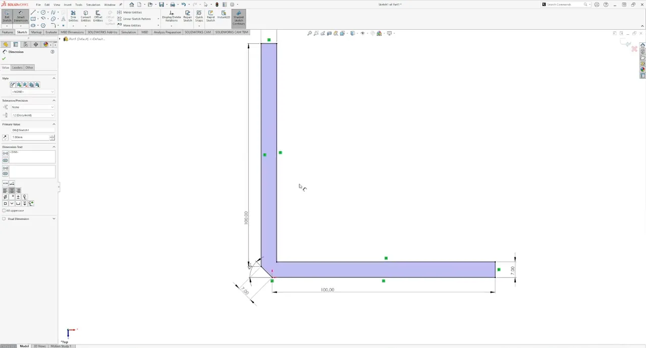
Both legs are \(100\) mm long with a square section of \(7 \times 7\) mm, and the outside of the corner is cut at \(45°\) (Figure 15.3.1). The inside corner is sharp. Sketch the profile on the Top Plane and extrude it \(7\) mm. The free end of the horizontal leg carries a force \(F\) perpendicular to the leg, in the plane of the L, and the end face of the vertical leg is fixed, as if glued to a wall.
A material for printed PLA
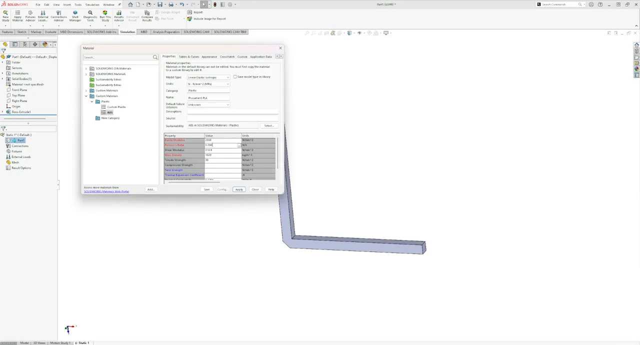
The SolidWorks library has no PLA. The default library is read-only, so we copy a similar plastic into a custom library and edit the copy. In the material dialog, open SOLIDWORKS Materials, Plastics, right-click ABS and Copy, then right-click Custom Materials, add a category Plastics and Paste. Rename the copy, here Prusament PLA, and enter the values of Figure 15.3.2. Creating a custom library needs write access to the folder where SolidWorks keeps it.
The values come from the manufacturer’s technical data sheet, and we have to read it with care. A filament manufacturer reports two kinds of strength. The tensile strength of the filament itself, a pulled length of wire, says little about a printed part. The strength of printed test bars, ISO 527 tensile specimens printed lying flat or standing on edge, is what we need. For Prusament PLA these give a tensile modulus of about \(2.3\) GPa and a yield strength of about \(50\) MPa, with an elongation at yield of a few percent, and the bars printed on edge are somewhat stronger than those printed flat, since more of their extruded lines run along the load. The strength across the layers is much lower. The yield point of PLA is itself a judgement: the tensile curve bends gradually, and where the straight part ends is the tester’s choice. PETG and nylon show no distinct yield point at all.
The study uses only the elastic modulus and Poisson’s ratio. Poisson’s ratio of the ABS copy, about \(0.39\), is close enough, and changing it hardly affects the stresses. The density matters only with gravity loads, and the tensile strength we enter only to have a reference line on the colour bar. We set \(E = 2300\) MPa and \(50\) MPa as the strength.
By using this material we assume that printed PLA is homogeneous, isotropic and linear elastic up to its yield strength. None of the three is true. A printed part has perimeters and infill, its stiffness and strength depend on the direction, and the tensile curve of PLA is linear only approximately and only over a small range. The study tells us where the bracket is stressed most and roughly how much, and no more.
Load, fixture and mesh
Fixtures, Fixed Geometry, on the end face of the vertical leg. External Loads, Force, on the end face of the horizontal leg, with Selected direction and an edge of the leg perpendicular to it as the direction, and Reverse direction if the arrow points the wrong way. We start with \(F = 50\) N, about the weight of \(5\) kg.
Create Mesh with a maximum element size of \(2\) mm. The section is \(7\) mm in every direction, so this gives at least two elements through it, and the part has no smaller features. The elements are second-order tetrahedra, the default.
Excessive displacements
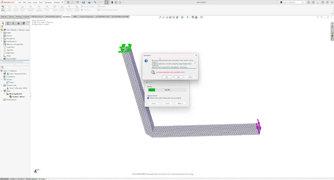
Run This Study, and SolidWorks stops with a message (Figure 15.3.3): Excessive displacements were calculated in this model. If your system is properly restrained, consider using the Large Displacement option to improve the accuracy of the calculations. Our system is properly restrained. The displacements are large because the bracket is slender, PLA is about ninety times more flexible than steel, and the load is large.
A hand estimate confirms it. The vertical leg, of length \(L = 100\) mm, carries the bending moment \(M = F a\) with the arm \(a \approx 96\) mm from its centre line to the force, and with \(I = 7^4/12 = 200~\text{mm}^4\) the corner rotates by
\[ \theta = \frac{ML}{EI} = \frac{50 \cdot 96 \cdot 100}{2300 \cdot 200} = 1.0~\text{rad} . \]
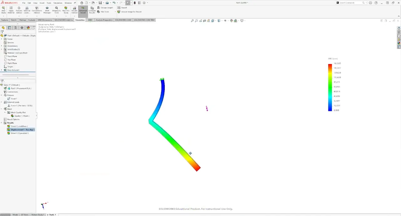
Small displacement theory assumes \(\theta \ll 1\), and a rotation of one radian, \(57°\), swings the free end by about \(100\) mm before the horizontal leg has bent at all. If we answer No and keep the linear solution, SolidWorks reports a displacement of \(162\) mm. With True scale in the Deformed Shape (Figure 15.3.4), the answer is plainly absurd. A linear model moves every point along a straight line, the tangent to its true path, so a large rotation also stretches the legs.
The stresses are also far beyond the \(50\) MPa of the material, so the bracket would not carry \(50\) N in any case. A linear static study does not know that. It is given only the slope of the tensile curve and extends it indefinitely, so a stress of several hundred MPa in PLA is a number the material never reaches, because it fails first.
We lower the force to \(5\) N and run again. The warning comes back, and this time we answer Yes. The study switches to large displacement theory, which applies the load in increments and updates the geometry after each, so the solution takes longer. The free end now moves \(15\) mm, and the hand estimate at \(5\) N is \(14\) mm, close enough for a problem that is still mildly nonlinear. The largest stress near the corner is about \(9\) MPa. With the beam formula, the bending stress at the corner is \(\sigma = M/W = 6Fa/b^3 = 6 \cdot 5 \cdot 96/343 = 8.4\) MPa.
The sharp corner
Once the study uses large displacement theory, it stays nonlinear: doubling the load no longer doubles the stress. We raise the load to \(F = 30\) N, for which the beam formula gives a nominal bending stress of about \(50\) MPa at the corner, right at the strength of the material. The highest stress sits along the inside corner. Plot Tools, Probe, On selected entities, select the edge of the inside corner and Update: the probe reports the stress at every node on the edge, with the maximum and the average.
We refine the mesh only along that edge, with Apply Mesh Control on the edge, and solve again for each size. Table 15.3.1 and Figure 15.3.5 show what happens.
| Element size at the corner | Max on the edge (MPa) | Average on the edge (MPa) |
|---|---|---|
| \(2\) mm (global) | \(70\) | \(59\) |
| \(0.5\) mm | \(128\) | \(93\) |
| \(0.1\) mm | \(262\) | \(202\) |
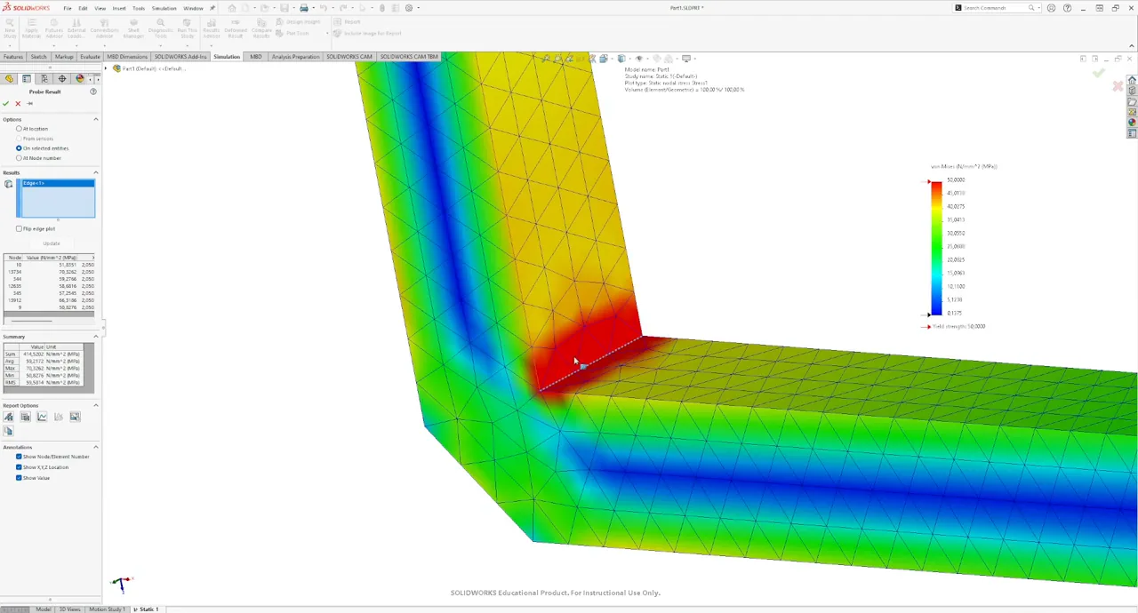
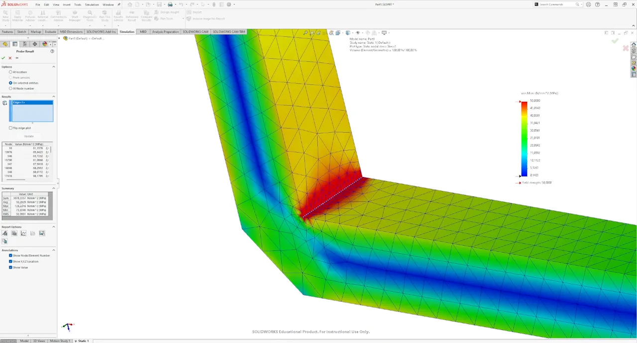
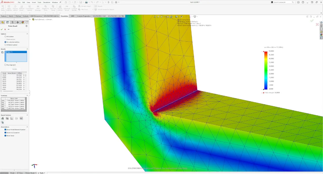
Each refinement roughly doubles the peak, and no mesh gives the answer. This is the stress singularity of Stress concentration or singularity: at a sharp re-entrant corner the stress of the elasticity solution grows without bound as we approach the corner, as \(\rho^{-0.46}\) for a right angle, and each element reports roughly the average over its own size. A finer mesh gives a larger number, and the model has no finite peak to converge to. An element size of \(0.1\) mm is also about ten times finer than anything used in practice, where \(1\) mm is a common lower limit, and the solution time grows quickly with every refinement, the more so in a nonlinear study that solves the system once per load increment.
Tension or compression
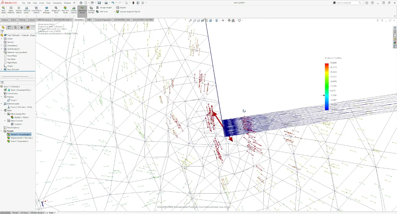
Von Mises is always positive, so its plot cannot tell whether the corner is pulled apart or pressed together. In Edit Definition, switch the component to P1, the first principal stress. Positive values are tension and negative values compression, and the plot shows tension at the inside corner, compression along the outside of both legs, and a neutral layer through the middle of each leg, where a beam in bending has no normal stress. Show vector plot draws each principal direction as an arrow (Figure 15.3.6). At the corner the arrows point away from each other, so the material there is pulled apart. Cracks open in tension and close in compression, so the bracket breaks at the corner. To inspect the compressed side, plot P3, the third and most compressive principal stress.
A fillet at the corner
Back in the model, add a Fillet of \(3\) mm to the inside corner. The old mesh control referred to the sharp edge and must be edited to refer to the fillet face. With a minimum of \(24\) elements around a circle, the probe over the fillet reports about \(50\) MPa in P1. Refined to \(0.1\) mm at the fillet the peak rises to \(65\) to \(67\) MPa and stays there (Figure 15.3.7). The value converges, so it is a stress concentration: a finite peak that the real part carries, and the place where a crack starts. Its ratio to the nominal \(50\) MPa is a stress concentration factor of about \(1.3\).
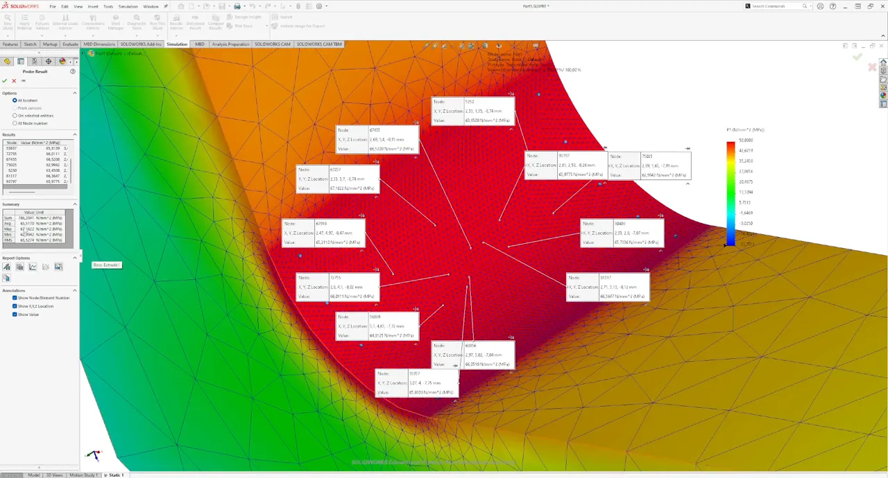
A \(1\) mm mesh would have shown the same picture. The sharp corner needed the refinement to reveal that it had no answer, and the fillet only needs a mesh fine enough to follow its curvature.
A fillet of \(10\) mm, meshed with \(1\) mm elements, lowers the stress further (Figure 15.3.8), to the strength of the material, so that \(30\) N, the weight of about \(3\) kg, is close to what the bracket can carry. The highest stresses now sit at the two ends of the fillet, where the arc meets the straight legs. A circular arc joins the legs with a tangent but with a jump in curvature, and transitions with gradually changing curvature lower the peak further.
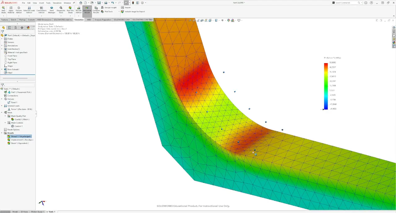
Without a fillet the study gives no load the bracket can carry, since the peak at a sharp corner grows with every refinement and a crack starts there in a real part too. With a fillet the same load gives a finite stress near the strength of the material. A printed corner is never perfectly sharp, since the extruded line rounds it, but that radius is a fraction of a millimetre and the peak is correspondingly high.
Printing the bracket
The P1 plot also tells us how to print the bracket. The tension at the inside corner runs along the legs, in the plane of the L, so the extruded lines should run there too. Printed lying flat, with the L in the plane of the bed, the perimeters follow the outline of the bracket and carry the tension along their length. Printed standing, with the L in a vertical plane, the tension at the corner pulls the layers apart, the direction in which printed PLA is weakest. The bracket is printed lying flat.
The study does not know any of this. It assumes a solid, homogeneous and isotropic material, with no infill and no layers, and a linear tensile curve with no yield point. Its results are most reliable for a metal loaded below its yield strength. For a printed part they locate the critical region and rank designs, a fillet against no fillet or one radius against another, faster than printing and testing each, and the test bars of the data sheet, or our own tests, set the strength we compare with.
Video
The bracket is worked through on screen, in Swedish, in Intro till Simulering.